How to Calculate Range in Google Sheets

When handling large amounts of data, being able to group certain values together can be very useful. Calculating hundreds of values automatically is one of the reasons that spreadsheets were made, after all. This is where being able to declare cell ranges is important, as it simplifies what would be otherwise cumbersome computations.

In this article, we’ll show you how to calculate range in Google Sheets, along with other handy Google Sheets range functions.

How to Find the Range in Google Sheets

The definition of a range in spreadsheets is quite different from its equivalent in math. Simply put, when working in spreadsheet programs, a range is a group of selected cells. This is important because by grouping cells together, you can use these groups as values for doing calculations. This allows a user to automatically compute formulas with a range as an argument.

Finding the range in Google Sheets is a very easy process. You just start from one end of a data set to the other. For example, a data set of ten numbers has a range either from one to ten or from ten to one. It doesn’t matter where you begin or where you end, as long as it covers the entire data set, that is your range.

If you look at the top and to the left of a Google Sheet document, you’ll notice that some letters and numbers mark them. This is how you determine the name of a particular cell in the sheet. You look at the letter from the top, then look at the number to the left. The very first cell would be A1, the cell immediately to the bottom of it would be A2, and the one to the immediate right is B2. This is how you determine the first and last value of your range.

Calculating the range would be easy if it was a single row or a column. Just use both ends of the data set that has a value then put a colon in between them. For example, in one column of data starting from A1 to A10, the range would be A1:A10 or A10:A1. It doesn’t matter if you use either end first.

It gets a little complicated when you’re working with multiple rows or columns. For this kind of data set, you need to determine two opposite corners to get your range. For example, a set of nine cells composed of three rows and three columns starting from A1 and ending at C3, the opposite corners would be A1 and C3 or A3 and C1.

It makes no difference whether you take the top leftmost and the bottom rightmost cells or the bottom leftmost and the top rightmost. As long as they’re opposite corners, you will cover the entire data set. The range would then be either A1:C3, C3:A1, A3:C1, or C1:A3. It doesn’t matter which cell you use as your first range value.

Finding the value of a range by typing in values is handy when the number of data values you have is too many to be able to select it manually. Otherwise, you can type in = in an empty cell, then click and drag your mouse over the entire data set to automatically generate a data range.

How to Create Named Ranges in Google Sheets

Named ranges become useful when you have too many range sets to keep track of. This can also help simplify calculations, as you can use the labels themselves as arguments for formulas. What’s easier to remember? =sum(a1:a10) or =sum(daily_sales)? By using the latter, not only will you know what the range is actually for, by looking at the formula alone you can see that the result is the sum of the day’s sales.

To create a named range, do the following:

1. Open your spreadsheet document in Google Sheets.
   
2. Select the range you want to name.
   
3. Click on Data on the top menu.
   
4. Click on Named ranges from the dropdown list. A window will pop up on the right.
   
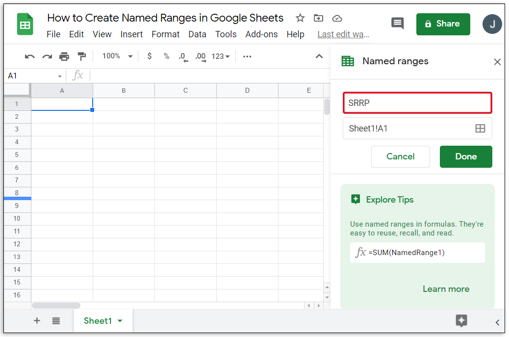
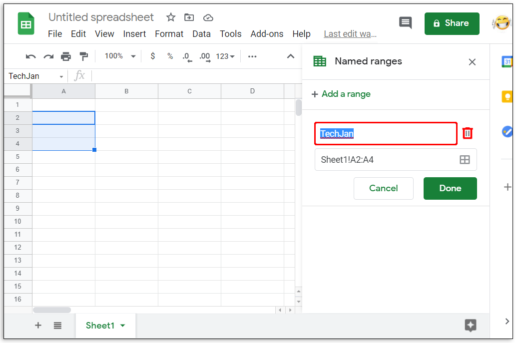
5. On the first textbox, type in the name that you want.
   
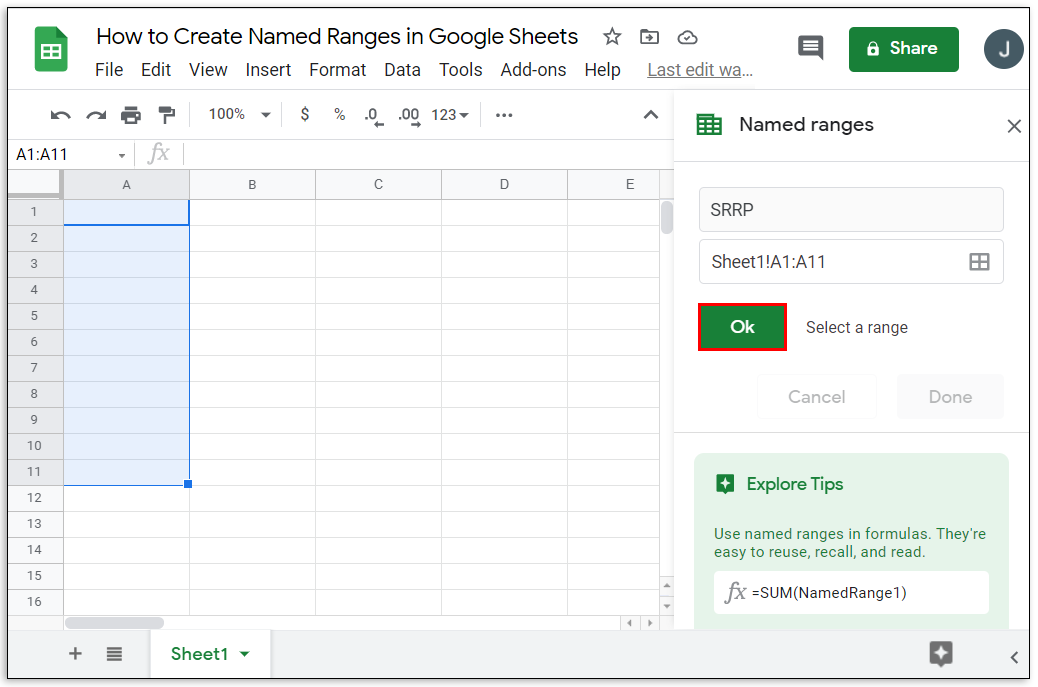
6. If you wish to change the selected range, you can change the values on the second textbox. If you have multiple sheets, you can type the sheet name followed by an exclamation mark (!) to specify which sheet you’re using. The values between colon (:) is the range.
   
7. Once you’re finished naming, click on Done.
   

There are certain rules that you must follow when naming ranges. Not adhering to these rules will often result in error messages or failure of a formula to produce a result. These rules are:

1. Range names can only contain numbers, letters, and underscores.
2. You can’t use spaces or punctuation marks.
3. Range names can’t begin with either the word true or false.
4. The name must be between one and 250 characters.

Here’s how to edit already named ranges:

1. Open the spreadsheets in Google Sheets.
   
2. Click on Data on the top menu.
   
3. Click on Named ranges from the dropdown menu.
   
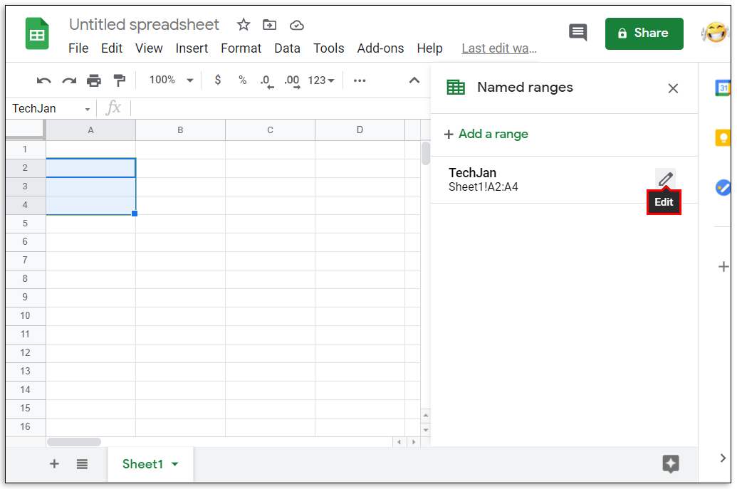
4. On the window to the right, click on the named range that you want to edit.
   
5. Click on the pencil icon to the right.
   
6. To edit the name, type in the new name then click on Done. To delete the range name, click on the trash can icon to the right of the range name, then click on Remove on the window that pops up.
   

Additional FAQs

How Do You Access AVERAGE Function in Google Sheets?

If you want to use the AVERAGE function, you can do the following:

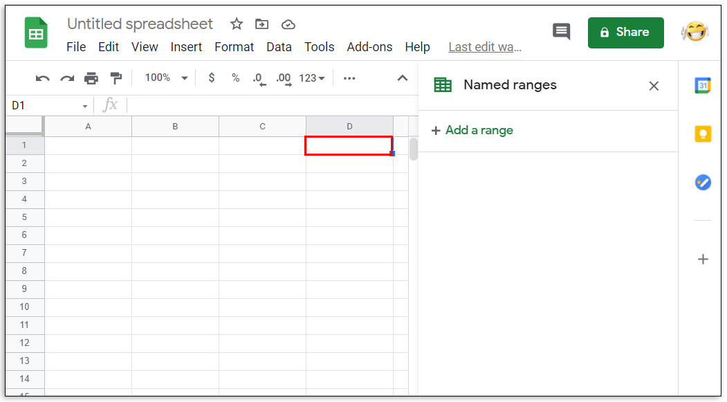
• Click on an empty cell where you wish the answer to be displayed.

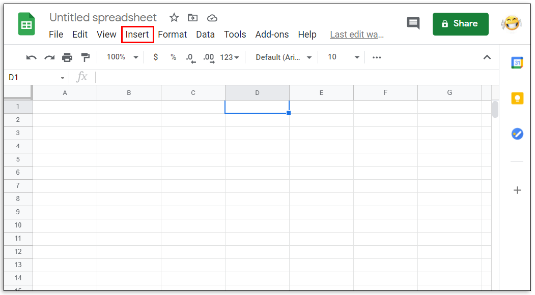
• On the top menu, click on Insert.

• Mouse over Function on the dropdown menu.

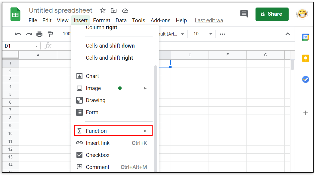
• Click on AVERAGE.

• Type in the values that you want the AVERAGE function to use.

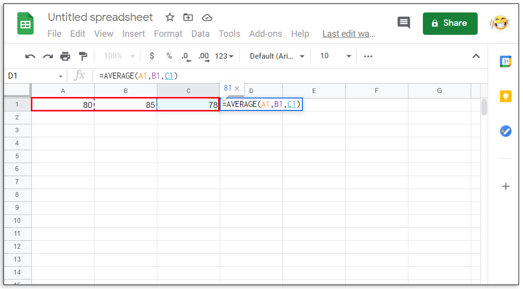
• Press the enter or return key.

How Do You Change Your Range in Google Sheets?

Changing the range is as easy as editing the first or last value of the cell numbers between the colon symbol. Remember that the range argument takes the first and last value you enter and includes all cells in between as a member of that range. Increasing or decreasing either number in between the colon will increase or decrease the members of the range accordingly.

How Do You Calculate Total in Google Sheets?

Formulas in Google Sheets can automatically calculate the total of a certain range of cells. If the values inside the cells are changed, the total will then adjust accordingly. The usual function used is SUM which is the total of all the values in the argument. The syntax of this function is =SUM(x:y) where x and y is the start and end of your range accordingly. For example, the total of a range from A1 to C3 will be written as =SUM(A1:C3).

How Do I Select a Data Range in Google Sheets?

You can select a range in two ways, either type in the range values manually, or click and drag your mouse over the entire range itself. Clicking and dragging is useful if the amount of data you have only spans a few pages. This becomes unwieldy if you have data that number in the thousands.

To manually select a data range, find the top leftmost value and the bottom rightmost value and place them in between a colon. The same also applies to the top rightmost and bottom leftmost values. You can then type this in as an argument in a function.

How Do You Find the Mean in Google Sheets?

In mathematical terms, the mean is the sum of the values of a set of cells, divided by the number of cells added. Simply put, it is the average value of all the cells. This can be accomplished by using the AVERAGE function in the Insert and Function menu.

What Is a Data Range in Google Sheets?

A data range is a set of cells that you want to use in a function or formula. It’s another name for range. The two names are interchangeable.

What Is a Valid Range in Google Sheets?

Depending on the formula you use, some values will not be accepted as an argument. For example, the cell value TRUE can’t be used in the formula =SUM() as it’s not a calculable numeric value. A valid range is a set of cells containing data that a formula will accept as an argument. If there is a cell that has an unaccepted input, then the range isn’t valid. Invalid ranges can also occur when either the first or last point of the range has a value that results in an error.

How Do I Find the Statistical Range of Values in Google Sheets?

In mathematics, the statistical range is the difference between the highest value and the lowest value of a set of data. Google Sheets has several functions that make the calculation of this rather simple. The MAX and MIN function is located under the Insert and Function menu. To find the statistical range or a data set just type in =(MAX(x) – MIN(x)) where x is your range. For the statistical range of a data set from A1 to A10, for example, the formula would be =(MAX(A1:A10) – MIN(A1:A10)). If you want rounded down values, you can use this syntax: =round(MAX(A1:A10),1)-round(MIN(A1:A10),1).

Efficient Calculations

Knowing how to calculate the range in Google Sheets helps users efficiently handle vast amounts of data. You can make use of all the formulas and functions that Google Sheets has to offer more easily if you can group data in specific sets and ranges. Understanding how ranges work can help simplify your workload.

Do you know of another way on how to calculate a range in Google Sheets? Share your thoughts in the comments section below.