How To Lock a Formula in Google Sheets

Matthew September 27, 2020

Google Sheets makes collaborating with coworkers on spreadsheets a snap with its easy sharing options. Unfortunately, when it’s that simple for multiple people to use the same spreadsheet, it’s also easy for a user to intentionally or unintentionally change critical formulas that the spreadsheet relies on. Actions can throw the whole sheet into chaos. The good news is that Google Sheets gives you a lot of control over permissions for users.

Locking cells is an excellent way to protect your spreadsheet formulas from unauthorized changes, ensuring that nobody can edit its functions. If you’re an Excel user, you might be interested in another article about locking Microsoft Office Excel formulas, but locking spreadsheet cells in Google Sheets is not performed the same way as it is done in Excel. Google Sheets formula protection does not require a password. Thus, you don’t need to enter a password to unlock cell protection to edit your own spreadsheets.

Regardless, Google Sheets doesn’t give you quite as many locking configuration options as Excel, but it features more locking formulas, which is more than sufficient in most cases. The “Protected sheets and ranges” tool locks a cell or range of cells from all editing, plus it has other custom options.

Lock a Full Sheet

If you want to allow viewing permission only (not editing) to other users, the simplest approach is to lock the entire sheet.

First, open the spreadsheet that includes the formula cells you need to lock. To protect all the cells within a spreadsheet, click the downward-pointing arrow on the sheet tab next to the name of the sheet at the bottom left of the spreadsheet and select Protect sheet, which will open the Protected sheets and ranges dialogue box as shown in the example below

Alternatively, you can also select the Protect sheet from the Tools pull-down menu. That will open the Protected sheets and ranges dialogue box as shown below.

In the Protected sheets and ranges dialogue box, follow these steps:

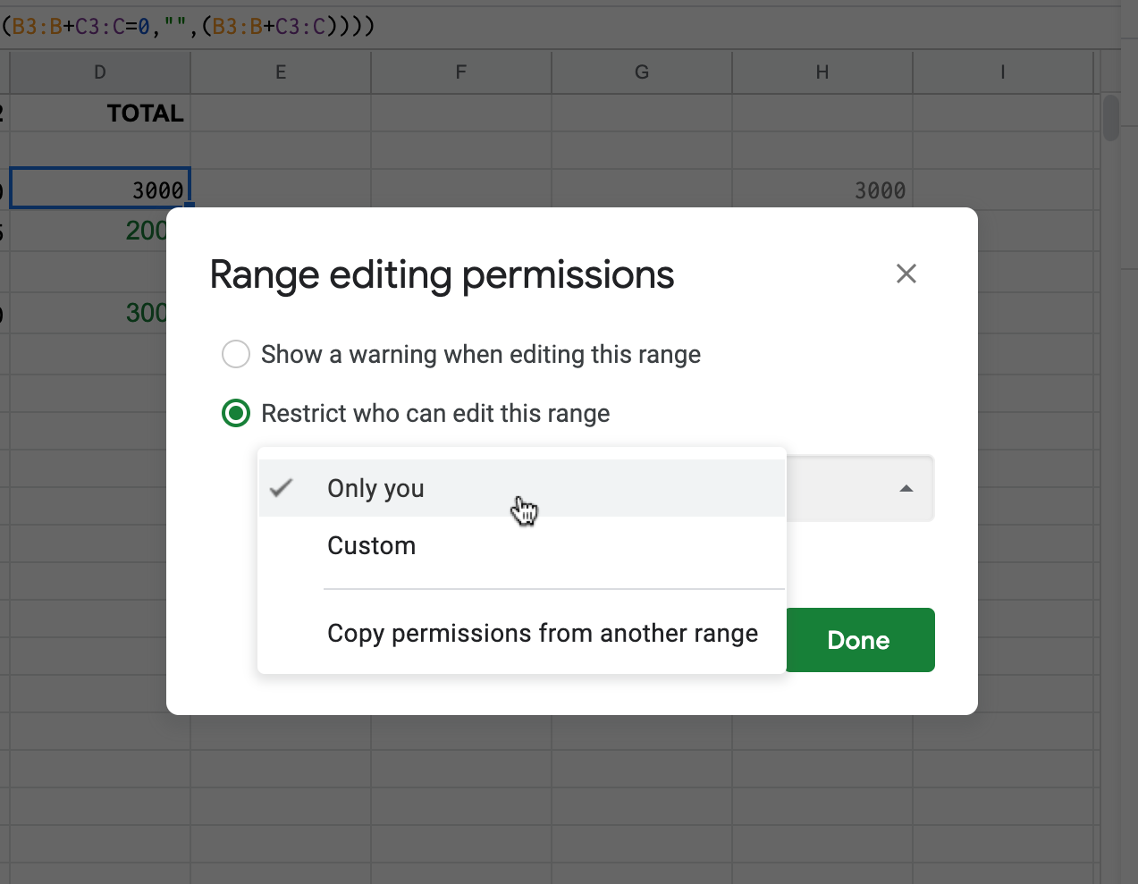
Press the Set Permissions button to open further editing permissions
Click the Restrict who can edit this range radio button
Then select Only you from the drop-down menu.
Press the Done to lock the spreadsheet

That will lock all the sheet’s cells for whomever you share it with. If somebody tries to modify a formula, an error message will open stating, “You are trying to edit a protected cell or object.”

Lock a Selected Cell or Cell Range

To protect formulas in various cells, you can select a range or select one cell at a time if they’re spread out in various locations on the sheet.

Note: If you select a cell that is already protected, the new entry will not work, leaving the cells editable by anyone with edit permissions. Be sure to check all currently protected cells first before selecting a new cell or cell range to protect.

If you only need to lock one or more formula cells in Google Sheets, follow these instructions:

Select the cell or range of cells you want to protect.
Click on “Data” in the top dropdown menu, then select “Protected Sheets and ranges.”
In the “Protected sheets & ranges” settings, select “Add a sheet or range.”
Create a name for the protected cell or cell range in the top box. Confirm the cells specified in the second box, which is already displayed if you selected them in the first step. Once completed, click “Set permissions.”
Choose your protection options in the “Range editing permissions” window. The warning option is a soft protection setting that allows editing but warns the user that is is not designed to be edited. The restricted option lets you choose who can edit the formula cell range. Click “Done” when satisfied with your settings.
Your new protection setting now displays in the “Protected sheets & ranges” settings on the right side of the sheet.

Changing/Editing Locked Cell Ranges and Their Settings

As an authorized editor, you have to request permission to edit protected formula cells and ranges by contacting the owner. As the owner, you can edit protected content by default, plus, you can edit existing protection settings.

If your protected cell ranges are not working and you need to edit them or find the “overlapping” cell(s) (as previously mentioned,) use the following steps.

To edit a protected entry, click the box for the item and the settings options will pop up. If you closed the toolbox already, go to “Tools -> Protected sheets and ranges.” Hit “Cancel” in the toolbox if it wants a new entry and it will go back to the protected list, as shown below.
If you selected an entry above for editing, you’ll get a new toolbox window that displays the entry’s name and cell range, as shown below. You can adjust the name and cell ranges here as needed. For user permissions, click on “Change permissions.”
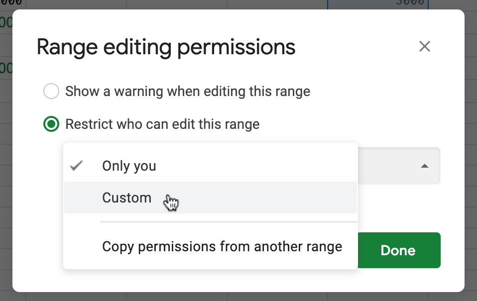
In the “Range editing permissions” window, adjust your user settings as needed.
If you chose “Custom” above, select who you want to receive edit privileges. You may need to repeat steps 1-3 above for other cell range entries, if applicable.
If you want to delete an entry, select it from the locked list, and then click on the trash can icon to select it for deletion.
A confirmation window will appear to authorize the deletion.

So that’s how you can ensure formulas in Google Sheets spreadsheets don’t get deleted or modified by unauthorized users. You might also enjoy this article on How to Get Absolute Value in Google Sheets.

Do you have any tips or tricks for protecting Google Sheets? Please comment below.