How to Calculate Age in Google Sheets from Birthdate

Google Sheets can be used for more than just data accumulation and organization. You can also use it to determine the current time, create charts, and calculate age using a birthdate. The latter is discovered through the use of formulas and functions built right into Google Sheets.

Follow along in this article to see how it’s done.

Determining Age from Birthdate in Google Sheets

When using Google Sheets, you have two predominant ways in which to determine age from a birth date. There’s DATEDIF, which is the more flexible option, and YEARFRAC, the simpler choice. By the end of the article, you should be able to determine not only the age of a single individual but that of multiple groups of varying people at once.

We’ll start things off with the DATEDIF function.

Calculating Age in Google Sheets using the DATEDIF Function

Before we can dive into the function itself, we’ll need to know how it works. This will take learning the syntax for use with the DATEDIF function. Each section you’ve typed in the Function correlates with a task, view these tasks below:

Syntax

=DATEDIF(start_date,end_date,unit)

• start_date
  • The calculation will have to begin with the birthdate.
• end_date
  • This will be the date to conclude the calculation. When determining the current age, this number will likely be today’s date.

• unit

• The output choices which consist of: “Y”,”M”,”D”,”YM”,”YD”, or “MD”.

• Y – Total number of full, elapsed years between both start and end dates entered.
  • YM – The ‘M’ stands for months. This output shows the number of months following the fully elapsed years for ‘Y’. The number will not exceed 11.
  • YD – The ‘D’ stands for days. This output shows the number of days following the fully elapsed years for ‘Y’. The number will not exceed 364.
• M – The total number of fully elapsed months between both start and end dates entered.
  • MD – As in the other units, ‘D’ stands for days. This output shows the number of days following the fully elapsed months for ‘M’. Cannot exceed 30.
• D – The total number of fully elapsed days between both start and end dates entered.

The Calculation

Now that you understand the syntax that will be used, we can set up the formula. As previously stated, the DATEDIF function is the more flexible option when determining age from a birth date. The reason for this is that you can calculate all the details of the age in a year, month, and day format.

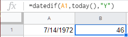
To begin, we’ll need an example date to use in the cell. We’ll be using 7/14/1972 for cell A1. We’ll be doing the formula in the cell to the right of it, B1, if you want to follow along to get the hang of it.

We’ll start with the most basic version of the formula to calculate the age. If you’re using the above syntax to figure out what is what, A1 is technically the start_date, today will be the end_date, and we’ll be determining the age in years using “Y”. That is why the first formula being used will look like this:

=datedif(A1,today(),"Y")

Helpful hint: Copy and paste the formula directly into B2 and hit Enter to receive the appropriate output.

When done correctly, the number, indicating the age calculated, will be situated in B1 as 46.

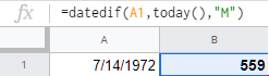
Let’s do the same formula only this time we’ll determine the age in months using “M” instead of “Y”.

=datedif(A1,today(),"M")

The total would be 559 months. That’s 559 months old.

However, this number is a bit absurd and I think we can take it down a notch by using “YM” in place of just “M”.

=datedif(A1,today(),"YM")

The new result should be 7, which is a much more manageable number.

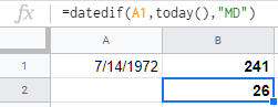
Just to be thorough, let’s see what the days will look like using both “YD” and “MD”.

=datedif(A1,today(),"YD")

=datedif(A1,today(),"MD")

This time the results for “YD” are shown in B1 and the result for “MD” is located in cell B2.

Got the hang of it so far?

Next, we’ll club these all together in an effort to provide ourselves with a more detailed calculation. The formula can get a bit hectic to type out, so just copy and paste the provided one into cell B1.

The formula to use is:

=datedif(A1,today(),"Y")&" Years "&datedif(A1,today(),"YM")&" months & "& datedif(A1,today(),"MD")&" days"

The ampersand is being used to join each formula together like a chain link. This is necessary to get the full calculation. Your Google Sheet should contain the same formula as:

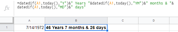
A full, detailed calculation has provided us with 46 Years 7 months & 26 days. You can also use the same formula using the ArrayFormula function. This means that you can calculate more than just a single date, but multiple dates as well.

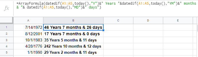
We’ve chosen a few dates at random and plugged them into additional cells A2-A5. Choose your own dates and have a little fun with it. To use the ArrayFormula function, copy and paste the following into cell B1:

=ArrayFormula(datedif(A1:A5,today(),"Y")&" Years "&datedif(A1:A5,today(),"YM")&" months & "& datedif(A1:A5,today(),"MD")&" days")

These are the results:

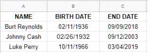
Now, let’s say that you wanted to separate each portion of the date into its own neat little column for organizing sake. In Google Sheets, add your start_date (the birth date) into one column and the end_date into another. We’ve chosen cell B2 for the start_date and C2 for the end_date in my example. My dates correlate to the births and recent deaths of celebrities Burt Reynolds, Johnny Cash, and Luke Perry.

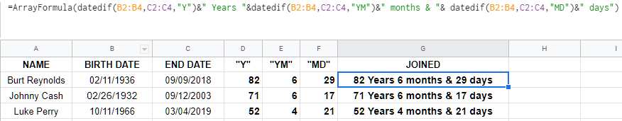
As shown, column A is the name of the individual, column B houses the start_date, and C the end_date. Now, we’ll add four more columns to the right. One for each of “Y”, “YM”, “YD”, and a combination of all three. Now you just have to add the correct formulas to each row for each celebrity.

Burt Reynolds:

=DATEDIF(B2,C2,"Y") Change ‘Y” to the corresponding column you’re trying to calculate.

Johnny Cash:

=DATEDIF(B3,C3,"Y") Change ‘Y” to the corresponding column you’re trying to calculate.

Luke Perry:

=DATEDIF(B4,C4,"Y") Change ‘Y” to the corresponding column you’re trying to calculate.

To get the JOINED formula, you’ll need to use an ArrayFormula just like we did earlier in the article. You can add words like Years to indicate the years’ results by placing it after the formula and in between parentheses.

=ArrayFormula(datedif(B2,C2,"Y")&" Years "&datedif(B2,C2,"YM")&" months & "& datedif(B2,C2,"MD")&" days")

The above formula is per celebrity. However, if you’d like to just knock them all out in one fell swoop, copy and paste the following formula into cell G2:

=ArrayFormula(datedif(B2:B4,C2:C4,"Y")&" Years "&datedif(B2:B4,C2:C4,"YM")&" months & "& datedif(B2:B4,C2:C4,"MD")&" days")

Your Google Sheet should end up looking something like this:

Pretty neat, huh? It really is that simple when using the DATEDIF function. Now, we can move onto using the YEARFRAC function.

Calculating Age in Google Sheets using the YEARFRAC Function

The YEARFRAC function is a simple one for simple results. It’s straight to the point providing an end result without all the extra added outputs for years, months, and days.

Here is a basic formula, applicable to only a single cell:

=int(YEARFRAC(A1,today()))

You’ll add the birth date to cell A1 and paste the formula into B1 for the result. We’ll use the birth date 11/04/1983:

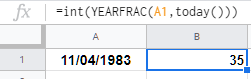
The result is 35 years of age. Simple, just like when using the DATEDIF function for a single cell. From here we can move onto using YEARFRAC within an ArrayFormula. This formula is more useful to you when you need to calculate the age of large groups like students, faculty members, team members, etc.

We’ll need to add a column of varying birth dates. For this, we’ll use column B as A will be used for the names of the individuals. Column C will be used for the end results.

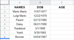
In order to populate the age on the adjoining column, we’ll need to use the following formula:

=ArrayFormula(int(yearfrac(B2:B8,today(),1)))

Place the formula above into cell C2 to get the results.

If you’d rather just proceed with an entire column and would rather not bother with figuring out where it ends, you can add a slight variation to the formula. Tack on IF and LEN toward the beginning of the ArrayFormula like so:

=ArrayFormula(if(len(B2:B),(int(yearfrac(B2:B,today(),1))),))

This will calculate all of the results within that column beginning from B2.

Google Sheets and Birthdates

Google Sheets has many useful built-in functions that can be used to make life easier. Whether it’s a function to quickly sum up values in a row/column or calculating someone’s age, Google Sheets has you covered.