Did you know your Excel sheet can have up to 1,048,576 rows? That’s right. Now imagine assigning numbers to each of these rows manually. We’re not talking about the existing numbers on the far left. Those are just markers, such as in relation to cells (A3, B3, A10, B10, etc.) that do not technically integrate as part of a row’s data, or serve as unique identifiers. What you want are numbers that can associate with each row of data for scenarios such as creating serial numbers or department numbers, applying numbered rows to grouped sections, etc.
To develop an excellent Excel worksheet or workbook, entering your data in a well-organized manner is imperative. You want each row to have a “unique identifier” that helps you single out specific rows for analysis or presentation to an audience. Using something like “Cell B4 or G2” is not tied to the data that spans the rows. You need columns that have unique numbers that actually tie into the data in the rows, just like the first name tying into the last name within the same row.
The good thing is that Excel can do all the hard work for you. You can command it to autofill row numbers and help you work on your document at a much faster pace.
This article will show you how to automatically number rows in Excel.
Reasons to Automatically Create Numbered Rows in Excel
Without a doubt, manually assigning row numbers is one task that can be frustrating and time-consuming. For starters, you might make mistakes and repeat numbers, a situation that can complicate data analysis and potentially result in errors in your calculations. Nothing is more embarrassing than presenting a document that’s poorly organized or laden with errors. It can make you look unprepared and unprofessional.
If your document is too large, you could assign numbers manually and make mistakes. But that’s hardly ever an option if your sheet has hundreds or thousands of rows or you have multiple spreadsheets and can’t use the same numbers. In that case, using rows A3 and B3, for instance, won’t cut it, especially when pulling data from several sheets for a report. Plus, manually numbering each one wastes valuable time you can spend on handling the more technical bits of your sheet.
One example includes department numbers or inventory classes, where you would want three digits for each one and start with 100. The problem is you have over 300 departments with data in 50 spreadsheets within your corporation. Manually typing the number identifiers into cells leads to mistakes that affect everything, from reports and data analysis to accurate categories and instant data retrieval. Rather than manually referring to 50 spreadsheets to determine and insert number identifiers for each row, you only need to remember what numbers you started and ended with so you can set up a different spreadsheet to have new identifiers or the same ones.
Another example is where you have groups of rows for specific topics, categories, departments, or even reference material. You want each group to start with number one. You certainly couldn’t reference “Cells A3 and B3” because you have groups on the same spreadsheet that can’t use the same row, but you can reference the identifiers 101 and 102 within each group and use them as often as needed. With so many groups to handle, manual entries quickly lead to mistakes that alter organization, data retrieval, and possibly priority levels where 1 is the most important and 1000 is the least.
Luckily, Excel comes with several tools designed to help you assign numbers automatically. This can help you to be more economical with your time and churn out a well-organized document that’s not only accurate but also easy on the eye. Pulling data from the spreadsheet/database is more manageable. Finding specific data or priority subjects/items/processes is precise and efficient without error.
The bottom line is that humans are not perfect when it comes to data entry, but automated systems guarantee preciseness and accuracy (to some extent). Whenever you have thousands of data entries, automatic numbering gets it done reliably.
Let’s see how each of these tools works.
Automatically Numbering Excel Rows Using the Fill Handle
The Excel Fill Handle, also called the Drag Fill Handle, is a small arrow button that appears in the bottom left corner of an active cell. It’s used to auto-populate a range of cells in a column based on information contained in the preceding rows.
The fill handle works by identifying a pattern and then following it.
Here’s how to automatically number rows in Excel using the fill handle.
- Open your Excel sheet.

- Enter the first value (1) into the first cell in the desired column.

- Enter the second value (2) into the cell directly below the first one.
- Select both cells.
- Press and hold on to the fill handle located in the bottom right corner of the lower cell.
- Gently drag down the handle until you’ve selected all the rows you’d like to assign numbers
- Once you get to the last row of interest, let go of your mouse.


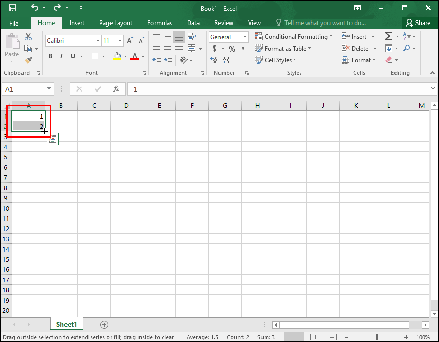
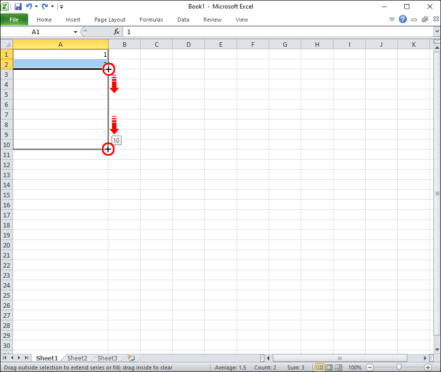

Upon completing the above steps, Excel populates all the cells in the chosen column with numbers, from “1” down to whatever number you want. These numbers become unique identifiers for the data in the row when A6 and B6 do not.
Automatically Numbering Excel Rows Using the ROW Function
The fill handle and the series function are simple to execute, but they fail in one crucial area: auto-updating numbers when you add new rows to your sheet or even remove some. The ROW function lets you assign numbers that automatically update whenever some rows are deleted, or new ones get inserted.
Here’s how to use the ROW function.
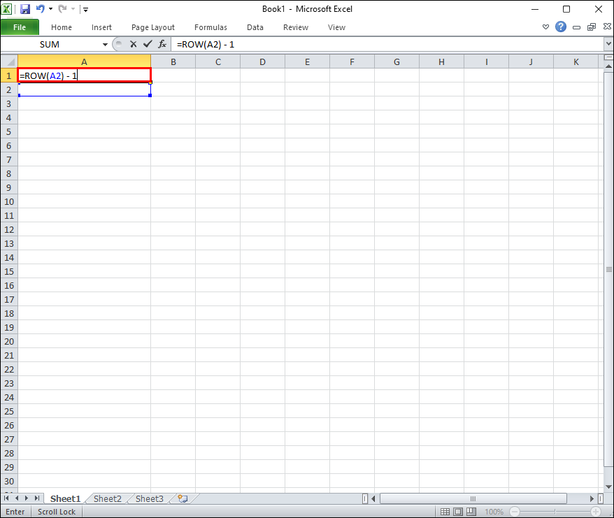
- Click on the first cell where the automatic numbering will begin.
- Enter the following formula into the cell (replace the reference row accordingly):
=ROW(A2) - 1.
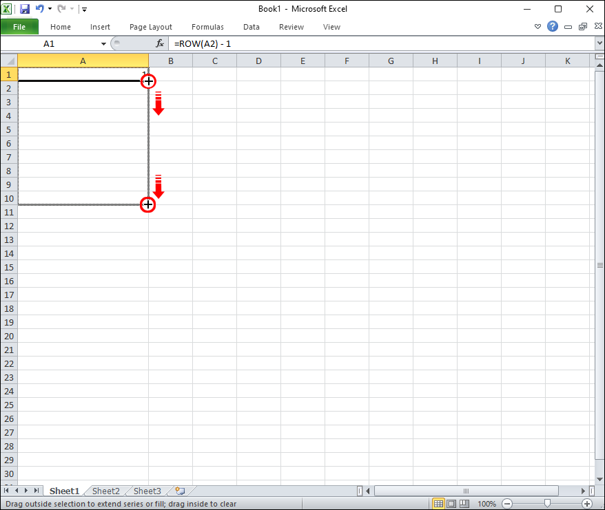
Depending on where you want your row numbers to begin, the formula could be A3, B2, or even C5. - Once a number has been assigned to the selected cell, hover the cursor over the drag handle in the bottom left corner, and drag it down to the last cell in your series.

How to Automatically Number Rows in Excel without Dragging
Dragging the fill handle down until you’ve selected all the rows you’d like to assign works ideally for small Excel files with just a few rows. If the file has hundreds or thousands of rows, dragging can be a bit tiresome and time-consuming.
Luckily, Excel provides a way to number your rows automatically using the “Fill Series” function.
The Excel Fill Series function is used to generate sequential values within a specified range of cells. Unlike the “Fill Handle” function, this one gives you much more control. You get to specify the first value (which need not be “1”), the step value, as well as the final (stop) value.
For example, let’s say your start, step, and stop values are 1, 1, and 10. The fill series feature auto-fills 10 rows in the selected column, starting with inserting “1” in the first cell, “2” in the second cell, etc., and ending with “10” in the last cell.
Here’s how to autofill row numbers in Excel using the Fill Series function:
- Select the first cell to which you’d like to assign a number.
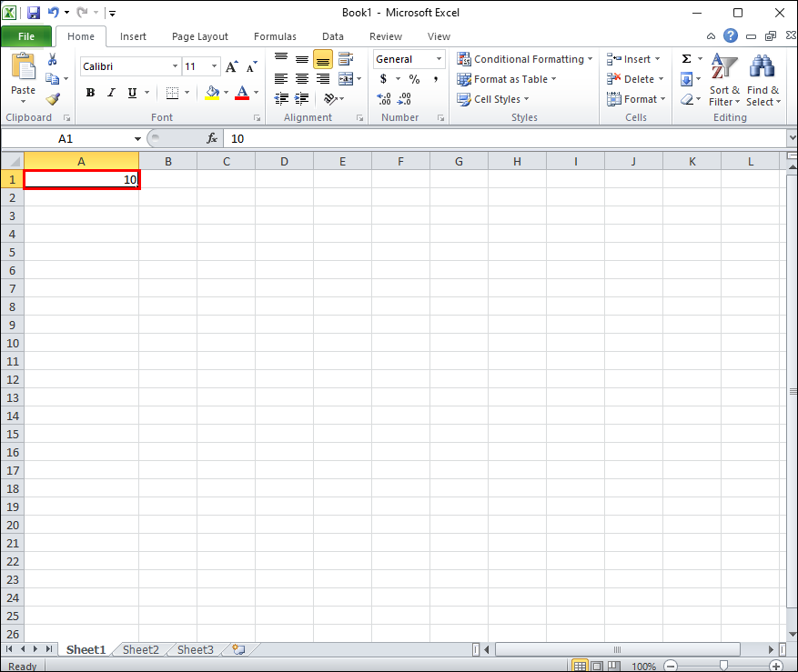
- Enter the first value, say “10,” in the first cell.
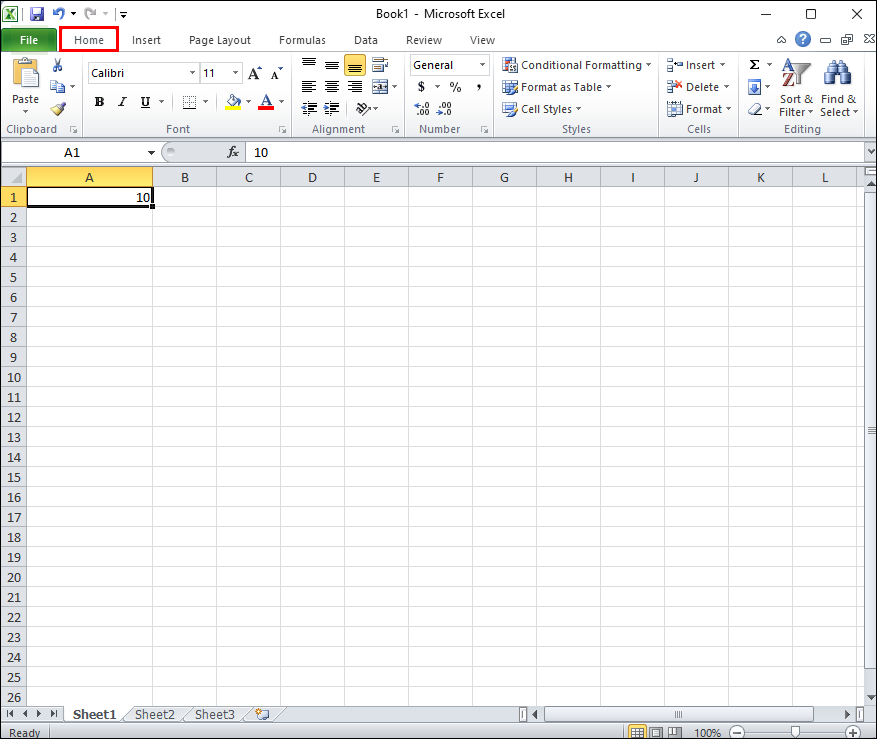
- Click on “Home” at the top of your sheet.
- Select “Fill” and then choose “Series” from the dropdown menu. This should open a floating dialog box in the middle of your sheet.
- In the dialog box, select “Columns” from the “Series in” section.
- At this point, enter the “step value” (“1” by default) and then enter the “stop value” in the spaces provided.
- Click on “Ok”


Upon completing the above steps, all the cells in the selected column get unique and sequential numbers for easy identification.
How to Automatically Number Filtered Rows in Excel
The “Filter” function allows you to sift (or slice) your data based on criteria. It enables you to select certain parts of your worksheet and have Excel show only those cells.
For example, if you have lots of repetitive data, you can easily filter out all of those rows and leave just what you need. Only the unfiltered rows appear on the screen at any given time.
When presenting data, filtering enables you to share just what your audience needs without having too much irrelevant information all at once. This situation can confuse and complicate data analysis.
Even if you’ve filtered your data, you can still add row numbering to your sheet.
Here’s how to go about it.
- Filter your data as needed.
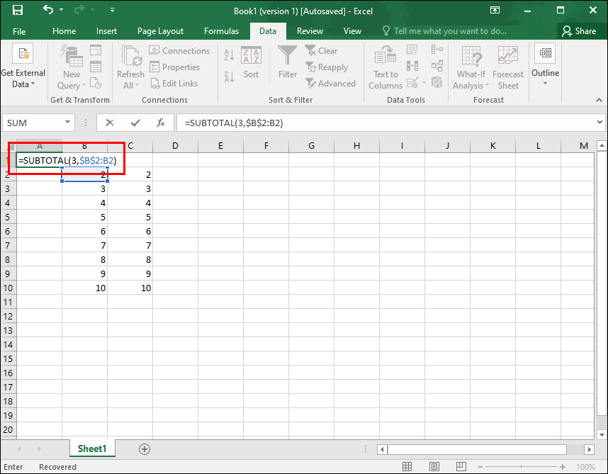
- Select the first cell to which you’d like to assign a number and then enter the following formula:
=SUBTOTAL(3,$B$2:B2)
The first argument, 3, instructs Excel to count the numbers in the range.
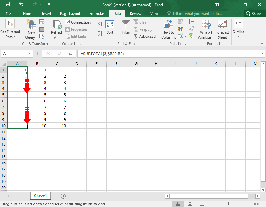
The second argument, $B$2:B2, is simply the range of cells you want to count. - Grab the “fill handle” (the plus symbol) in the bottom right corner of the cell and pull it downwards to populate all the other cells in the specified range.

Overall, Excel is a valuable tool for managing data and performing all sorts of calculations, but it doesn’t always make life easy. One task that can be time-consuming and frustrating is assigning numbers to rows, especially with thousands of them or when several spreadsheets exist.
Fortunately, there are several tools to help you assign numbers automatically. This can be a surefire way to create a well-organized database that’s easy to read, easy to retrieve specific data, and easy to create accurate reports and statements.
Disclaimer: Some pages on this site may include an affiliate link. This does not effect our editorial in any way.