Google Sheets is similar to Microsoft Excel and many of Excel’s features are replicated or mirrored inside Sheets, making it easy to make the switch from Microsoft’s productivity suite to Google’s own offerings. Users with basic spreadsheets (those without custom macros or design elements) can in fact just directly import their Excel files into Sheets without any problems or glitches.
One problem that spreadsheet users have had is that in the process of importing and collating data from multiple sources (one of the many tasks that spreadsheets are great at), it is not at all uncommon for random empty cells, rows, and columns to appear inside the document. Although this problem is manageable in smaller sheets, where you can just delete the rows manually, it’s a huge problem when it crops up in larger documents.
However, removing these blank spaces is quick and easy if you know the proper steps. In this article, we’ll show you how to remove all the empty rows and columns in your Google Sheets document using an auto-filter.
Deleting Empty Rows and Columns in Google Sheets using the Keyboard Shortcut
If you’re trying to delete all of the empty rows below your content, you can.
- To get rid of all the empty columns simply click on the row you’d like to start with and use the following keyboard command:
- On a Mac press Command + Shift + Down Arrow.
- On Windows press Control + Shift + Down Arrow.
- Once you’ve done this, you’ll notice the entire sheet is highlighted. Right-click and select the option to delete all rows. Your finished product will look like this:
You can do the same for all the columns to the right of your data as well. Using the same commands as above, use the Right Arrow, highlight all columns, right-click, and delete. This leaves a much cleaner looking datasheet.
Deleting Empty Rows and Columns using the Auto-Filter
Put simply; an auto-filter takes the values inside your Excel columns and turns them into specific filters based on the contents of each cell—or in this case, the lack thereof.
Though originally introduced in Excel 97, auto-filters (and filters in general) have become a massive part of spreadsheet programs, despite the small minority of users who know about and use them.
Setting Up an Autofilter
The auto-filter function can be used for a number of different sorting methods. In fact, they’re powerful enough to sort and push all of the empty cells to the bottom or top of your spreadsheet.
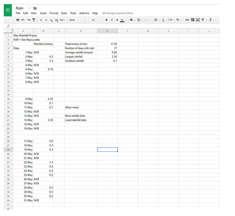
- Start by opening up the spreadsheet that contains empty rows and columns you want to remove from your document.
- Once the document has opened, add a new row at the very top of your spreadsheet. In the first cell (A1), type whatever name you’d like to use for your filter. This will be the header cell for the filter we’re about to create.

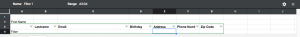
- After creating the new row, find the Filter icon in the command row inside Google Sheets. It’s pictured below; its general appearance is similar to an upside-down triangle with a line running out the bottom, like a martini glass.
- Clicking this button will create a filter, which will by default highlight a few of your cells in green on the left side of the panel.
- Because we want this filter to extend to the entirety of our document, click the small drop-down menu next to the filter icon. Here, you’ll see several options for changing your filters. At the top of the list, select Create new filter view.
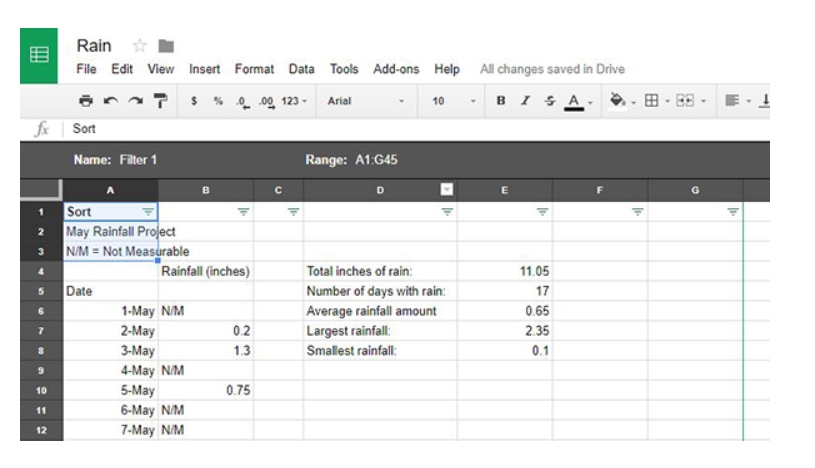
- Your Google Sheets panel will extend and turn a dark grey color, along with an entry point for you to insert the parameters of your filter. It’s not critical that you include every single column, but ensure that you’ve included every row and column in your document that contains blank spaces.


To be safe, you can just have the filter cover the entirety of your document. To input this into your document, type something like A1:G45, where A1 is the starting cell and G45 is the ending cell. Every cell in between will be selected in your new filter.
Using the Autofilter to Move Blank Cells
This next bit may seem a bit odd because it will be moving and reorganizing your data in a way that seems counterintuitive at best and destructive at worst.
- Once your filter has been selected, click the green triple-line icon in the A1 column of your spreadsheet where you set a title earlier.
- Select Sort A-Z from this menu. You’ll see the data move into alphabetical order, beginning with numbers and followed by letters, also, the blank spaces will be pushed to the bottom of your spreadsheet.
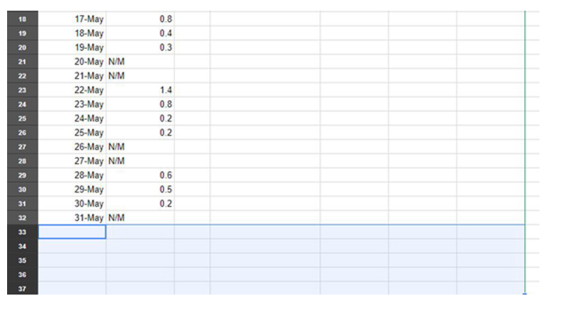
- Continue to resort your spreadsheet column by column until your blank cells have moved to the bottom of the display and you have one solid block of data displayed at the top of Google Sheets.

This will likely make your data a confusing, unreadable mess—don’t worry, this will all work out in the end.
Deleting Your Blank Cells
Once your blank cells have been moved to the bottom of your spreadsheet, deleting them is as simple as deleting any other cell.
- Use your mouse to highlight and select the blank cells on your spreadsheet that have been moved to the bottom of the document. Do this by clicking and holding the left mouse button and drag the cursor over the blank cells.
- Depending on the number of blank cells and the working area of your spreadsheet, you might want to zoom out of your display a bit to see more of the surrounding area (most browsers, including Chrome, allow you to zoom by using Ctrl/Cmd and the + and – buttons; you can also hold down Ctrl/Cmd and use the scroll wheel on your mouse or touchpad).
- Once highlighted, simply right-click to delete the blank cells.
Reorganizing Your Spreadsheet
Now that you’ve removed the offending blank cells, you can reorganize your spreadsheet back to normal order. While clicking on that same triple-lined menu button from earlier inside the filter will only allow you to organize in alphabetical or reverse alphabetical order. There is another sort option: turning your auto-filter off.
- To do this, click the triangle menu button next to the auto-filter icon inside Sheets.
- Inside this menu, you’ll see an option for your filter (called Filter 1, or whatever number filter you’ve made), as well as an option for None. To turn off the filter you applied earlier, simply select None from this menu.
Your spreadsheet will return to normal like magic but without the blank cells, you deleted earlier.
With the cells deleted, you can resume reorganizing and adding data back into your spreadsheet. If, for whatever reason, this method causes your data to fall out-of-order, reversing it is as simple as diving into your documents’ history and reverting to an earlier copy.
You can also use the copy and paste function to move your data around easily, without having to deal with hundreds of blank cells blocking your path. This isn’t a perfect solution but it does work to push your data above the mass of blank cells in your document. And at the end of the day, it’s a lot easier than mass-deleting rows one by one.
Disclaimer: Some pages on this site may include an affiliate link. This does not effect our editorial in any way.