How To Delete Hidden Rows in Google Sheets

Google Sheets is a handy tool for creating and editing spreadsheets. It offers numerous useful features, and one of them is hiding cells. Many people use this feature because it enables them to temporarily remove irrelevant cells from the spreadsheet. If you’ve received a spreadsheet with hidden rows and realized you don’t need them, you can easily delete them without jeopardizing the rest of the data.

This article will show you how to delete hidden rows in Google Sheets using numerous devices.

Delete Hidden Rows in Google Sheets on a PC

Even though Google Sheets is very similar to Microsoft Excel, it differs when it comes to deleting hidden rows. We’ll show you two ways of deleting these rows. The one you should use depends on what method was used to hide them.

How to Delete Hidden Rows in Google Sheets on a PC: Method One

If you’re looking at a spreadsheet and notice some of the rows are missing, you first need to establish how they were hidden. There are two ways of hiding rows: directly from the sheet or with filters.

Here’s how to check this:

1. Launch Google Sheets.
   
2. Open the sheet in question.
   
3. Right-click the gray block at the top-left corner of the sheet.
   
4. Look at the “Unhide rows” option. If it’s grayed out, rows weren’t hidden with the “Hide row” option. If the option is clickable, it means the rows were hidden using this option. Here, we’ll discuss how to unhide them.
   

The typical tell-tale signs for rows hidden in this way are two arrows in consecutive rows. To delete such rows, you’ll first need to unhide them:

1. Press one of the arrows. The hidden rows will automatically appear on the sheet as highlighted.
   
2. Right-click on the highlighted row.
   
3. Press “Delete row.”
   

Repeat this action for all hidden rows you wish to delete.

How to Delete Hidden Rows in Google Sheets on a PC: Method Two

In some cases, you may notice some row numbers are missing, but there are no arrows next to them that would indicate the rows have been hidden. This usually means the rows were filtered. When you don’t see the arrows, look for filter icons on the right of some column headers. These icons look like funnels.

Here’s how to delete filtered rows:

1. Press the filter icon.
   
2. Under the search bar, you’ll see checked and unchecked data. The checked data is visible in the sheet, while the unchecked data represents filtered or hidden rows. You need to reverse this by checking the rows you want to delete and unchecking the ones you wish to keep.
   
3. Now, the “hidden” rows will appear in the sheet while the ones you want to save are hidden. Select the row numbers on the left and press “Delete selected rows.”
   
4. Press the filter icon again and check the remaining rows to display them in the spreadsheet.
   

Delete Hidden Rows in Google Sheets on an iPhone

The Google Sheets mobile app is available on iPhones and enables users to create, view, and edit spreadsheets. If you’ve noticed a spreadsheet has hidden rows and want to remove them permanently, you can use one of two methods. Keep in mind that the method you choose will depend on how the rows were hidden.

How to Delete Hidden Rows in Google Sheets on an iPhone: Method One

If you’ve noticed inconsecutive row numbers in your spreadsheet, it means some of the rows are hidden. This method shows you how to delete rows that were hidden using the “Hide row” option. The two arrows in place of the hidden rows will indicate if this is the case. If you don’t see the arrows, jump to the second method.

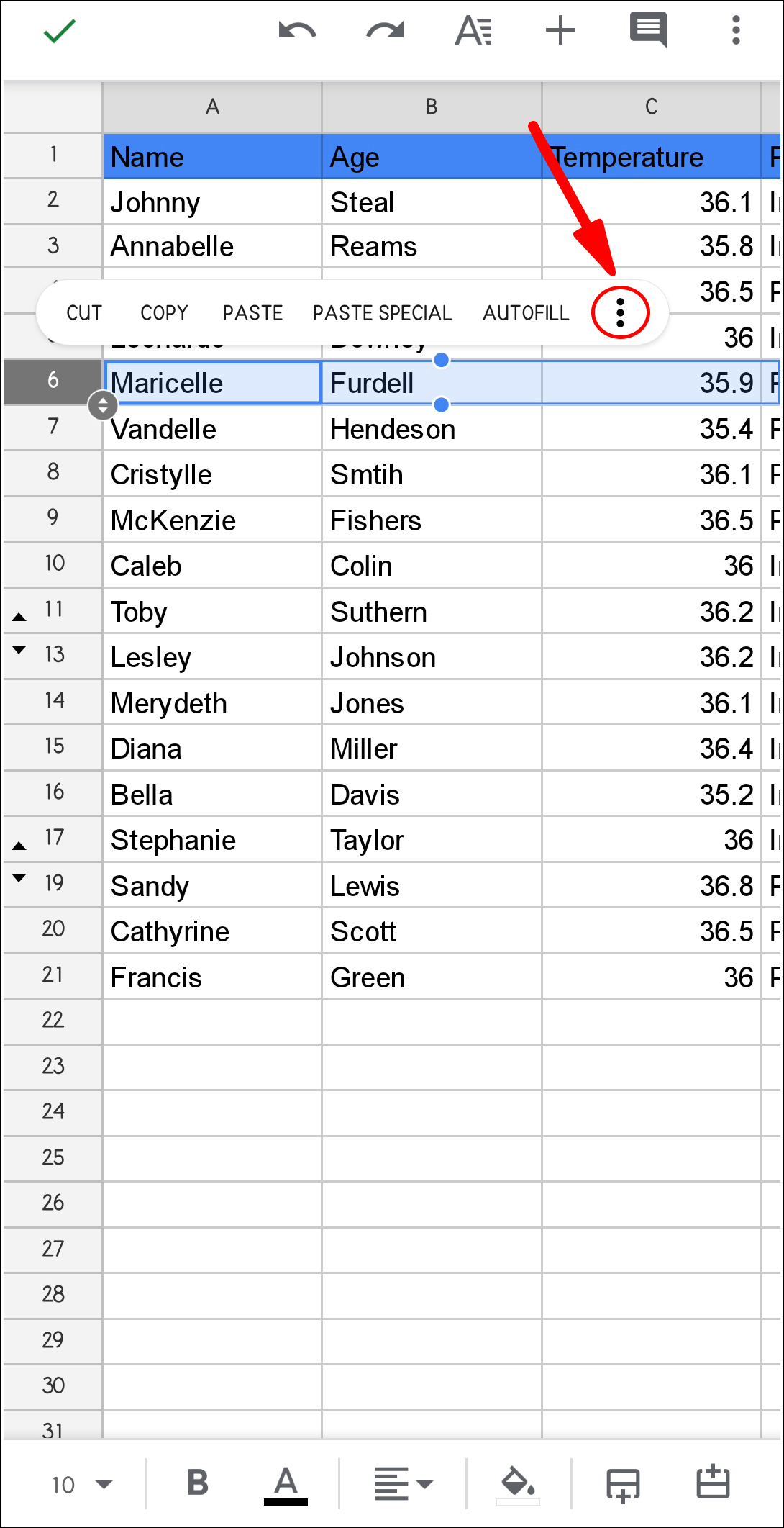
Here’s how to delete hidden rows on your iPhone:

1. Tap the arrows in place of the hidden row. The row will reappear in the sheet. You don’t have to remember its position since it will be highlighted.
   
2. Tap and hold the highlighted row and press the three dots.
3. Tap “Delete.”
   

Repeat the process as necessary.

How to Delete Hidden Rows in Google Sheets on an iPhone: Method Two

If you’ve noticed row numbers aren’t consecutive and don’t see the arrows next to where the rows should be, it means they are filtered. In that case, you’ll see a green filter icon in the column heading.

Follow the steps below to delete filtered rows in Google Sheets using an iPhone:

1. Tap the green filter icon in the column heading. Data with a checkmark represents visible information, i.e., the information you want to keep. Unselect the data, and select only the rows you want to delete.
2. The spreadsheet will now display the rows that were previously hidden. Select them by tapping and holding their number, tap the three dots, and press “Delete.”
3. Tap the filter icon and select the rows you want to display again or tap “Select all.”

Delete Hidden Rows in Google Sheets on an Android

Android users will be happy to know that they can use their phones to delete hidden rows in Google Sheets. Two methods can be used for this, and the option you’ll choose will depend on how the rows were hidden. Namely, Google Sheets offers the “Hide row” option, but it also enables users to apply filters to hide the rows. The first method explains how to delete hidden rows, while the second discusses deleting filtered rows.

How to Delete Hidden Rows in Google Sheets on an Android: Method One

If the rows in your spreadsheet were hidden using the “Hide row” option, you’ll see small arrows that indicate their position.

Follow the instructions below to delete these rows:

1. Tap one of the small arrows to unhide the row. The unhidden row will appear in the spreadsheet. You don’t have to memorize its exact position, because it will be highlighted.
   
2. Press and hold the row and tap the three dots on the right.
   
3. Tap “Delete.”
   

Keep in mind that this option doesn’t delete all hidden rows in a spreadsheet. If you want to delete all of them, you’ll need to repeat the process wherever you notice the small arrows.

How to Delete Hidden Rows in Google Sheets on an Android: Method Two

Sometimes, you may notice inconsecutive row numbers, but there will be no small arrows that indicate some of the rows are hidden. This means the rows were removed from the spreadsheet using a filter. In such cases, you’ll notice a green filter icon in a column heading.

Here’s how to delete filtered rows in Google Sheets using your Android phone:

1. Find and select the green filter icon in a column heading. Pay attention to the checked and unchecked data. The latter represents filtered or “hidden” rows you want to delete. To do this, you’ll need to check them while unchecking the data you want to keep.
2. The spreadsheet will now show only the rows you want to delete. Select them, tap the three dots on the right, and choose “Delete.” Once you do this, you’ll end up with an empty spreadsheet.
3. Select the filter icon again, and check the rows you want to display in the spreadsheet. You can also use the “Select all” option.

Delete Hidden Rows in Google Sheets on an iPad

Many people enjoy using Google Sheets on their iPads because of the larger screen. As with other devices, there are two ways of deleting hidden rows in Google Sheets, and we’ll cover both.

The method you choose depends on whether the rows were actually hidden or filtered. Let’s start with hidden rows.

How to Delete Hidden Rows on an iPad: Method One

Signs that indicate hidden rows in Google Sheets are inconsecutive numbers and small arrows that mark their position. Follow the steps below to delete such rows:

1. Scroll through the spreadsheet to locate small arrows representing the hidden row and tap them. The row will now be unhidden and highlighted.
   
2. Tap and hold the number of the highlighted rows and select the three dots on the right.
3. Press “Delete.”
   

Repeat the steps for all hidden rows you wish to permanently remove from the spreadsheet.

How to Delete Hidden Rows on an iPad: Method Two

Another way to hide rows in a spreadsheet is by using filters. Such rows aren’t marked with small arrows but filter icons in column headings. This may sound complicated at first, but deleting filtered rows is usually much easier since you don’t have to do it one by one.

Here’s how to remove filtered rows from your spreadsheet using an iPad:

1. Locate the filter icon in one of the column headings and tap it. The icon looks like a funnel. The unchecked data represents the “hidden” rows, i.e., the rows you want to delete. Check those rows and uncheck the ones you need to keep.
2. The spreadsheet will now show only the rows that were previously hidden. Select the rows, press the three dots, and tap “Delete.”
3. Tap the filter icon again and check the rows you want to see in the spreadsheet, or use the “Select all” option.

Hidden Rows Can Cause Trouble

Just because you have hidden rows in Google Sheets doesn’t mean their values are gone. If you’ve applied a formula on such rows, the numbers will be factored in even if you can’t see them on the sheet. This can be especially confusing if you share the sheet with your coworkers.

We hope this article helped you learn how to delete hidden and filtered rows in Google Sheets and avoid further confusion.

Do you often use the “hide row” option in Google Sheets? Did you ever forget to unhide or delete such rows? Tell us in the comments section below.