How To Freeze Multiple Rows in Excel

If you’re a data enthusiast, you’ve probably had to analyze tons of data stretching hundreds or even thousands of rows. But as the data volume increases, comparing information in your workbook or keeping track of all the new headers and data titles can be quite an uphill task. But that’s exactly why Microsoft has come up with the data freeze feature.

As the name suggests, freezing holds in place rows or columns of data as you scroll through your worksheet. This helps you to remember exactly what kind of data a given row or column contains. It works pretty much like using pins or staples to hold large bundles of paper in an orderly, organized manner.

How to Freeze a Single Row on Excel

First, let’s see how you can freeze a single row of data. This is usually the top row in your workbook.

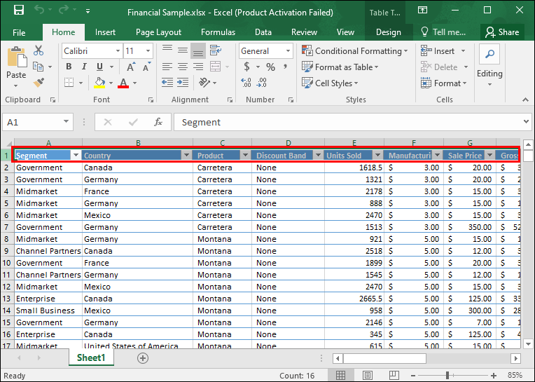
1. Open the Excel worksheet and select the row you wish to freeze. To do so, you need to select the row number on the extreme left. Alternately, click on any cell along the row and then press “Shift” and the spacebar.
   
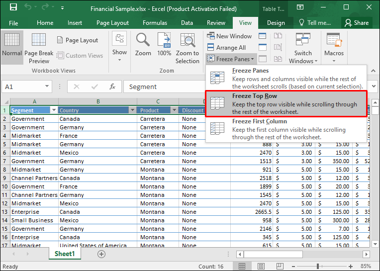
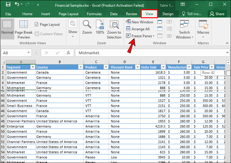
2. Click on the “View” tab at the top and select the “Freeze Panes” command. This will create a dropdown menu.
   
3. From the options listed, select “Freeze Top Row.” This will freeze the first row, no matter what row you happen to have currently selected.
   

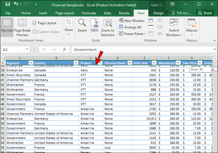
Once a row has been frozen, Excel automatically inserts a thin gray line below it.

If you wish to freeze the first column instead, the process is pretty much the same. The only difference is that this time you’ll have to select the “Freeze First Column” command on the dropdown list at the top.

How to Freeze Multiple Rows

In some instances, you may want to lock several rows at once. Here’s how to do this:

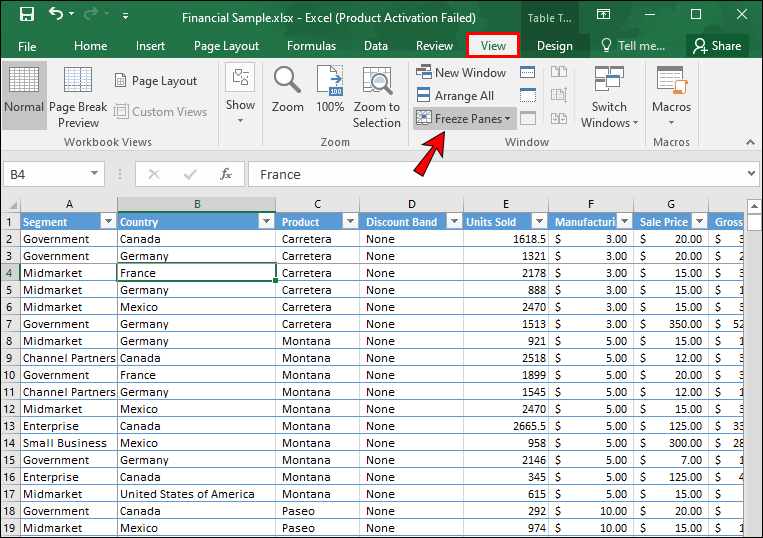
1. Select the row immediately below the rows you want to lock. As before, clicking on any cell in the row and pressing “Shift” and the spacebar will do the trick.
   
2. Click on the “View” tab at the top and select the “Freeze Panes” command.
   
3. From the resulting dropdown list, select the “Freeze Panes” command. In recent MS Excel versions, this option takes the top spot on the dropdown list.
   

Again, Excel automatically inserts a thin line to show where the frozen pane begins.

How to Unfreeze Panes

Sometimes you may end up freezing a row unintentionally. Or, you may want to unlock all rows and restore the worksheet to its normal view. To do so,

1. Navigate to “View” and then select “Freeze Panes.”
   
2. Click on “Unfreeze Panes.”
   

Additional FAQs

I can’t see the “Freeze Panes” option. What’s the problem?

When you have been working on a large worksheet for a while, it’s possible to lose track of changes you’ve made to your document over time. If the “Freeze Panes” option is not available, it may be because there may be panes that are frozen already. In that case, select “Unfreeze Panes” to start over.

Are there alternatives to freezing?

Freezing can be quite helpful when analyzing huge chunks of data, but there’s a catch. You can’t freeze rows or columns in the middle of a worksheet. For this reason, it is important to familiarize yourself with other view options. In particular, you may want to compare different sections of your workbook, including sections in the middle of the document. There are two alternatives:

1) Opening a New Window for the Current Workbook

Excel is equipped to open as many windows as you wish for a single workbook. To open a new window, click on “View” and select “New Window.” You can then minimize the dimensions of the windows or move them around as you like.

2) Splitting a Worksheet

The split function allows you to break up your worksheet into multiple panes that scroll separately. Here’s how you perform this function.

• Select the cell where you want to split your worksheet.

• Navigate to “View” and then select the “Split” command.

The worksheet will be split into multiple panes. Each one scrolls separately from the others, allowing you to scrutinize different parts of your document without having to open multiple windows.

Freezing multiple rows or columns is a straightforward process, and with a bit of practice, you can lock any number of rows. Have you encountered any errors while attempting to freeze multiple rows in your documents? Do you have any freeze hacks to share? Let’s engage in the comments.