How to Highlight Values That Are Greater or Less Than in Microsoft Excel

Highlighting certain sections across a large data set can help you acquire some valuable insights from the data you’re currently working on. For instance, you might want to highlight values that are greater or less than a specific number in your Excel documents in order to make critical judgments.

However, manually doing it is time-consuming and a recipe for errors. This article highlights how you can go about the process using conditional formatting.

How to Highlight Values That Are Greater or Less Than in Excel

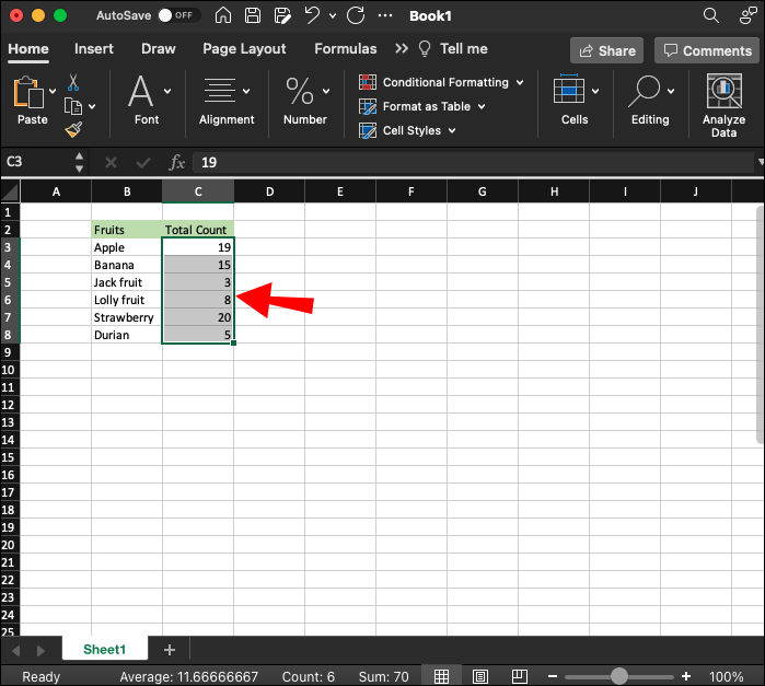
Highlighting certain values across your spreadsheet makes it easy to pinpoint what you’re looking for, making data analysis a breeze. To highlight certain sections of a spreadsheet, we use an Excel feature called conditional formatting. As the name suggests, the feature works by letting you alter the appearance of specific data items if they meet a predefined condition. As a result, this makes them easier to identify, especially if you have a large data set.

How to Highlight Values That Are Greater or Less Than a Specific Number in Microsoft Excel

Here’s how to highlight values that are greater than a specific number in Microsoft Excel:

1. Open the Excel sheet whose values you’d like to highlight. Choose the range of cells you want to work on by dragging the mouse over them.
   
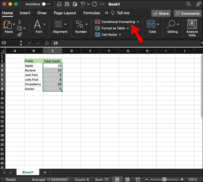
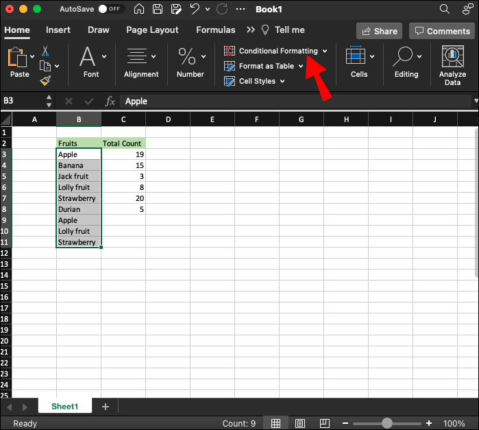
2. On the homepage, click on the “Conditional Formatting” menu.
   
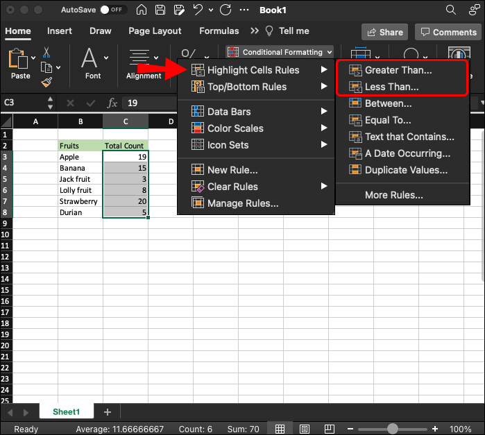
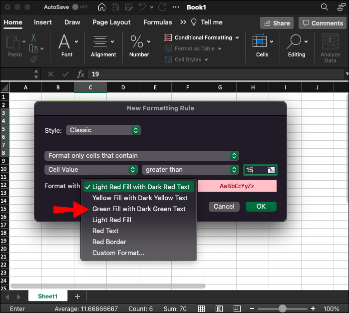
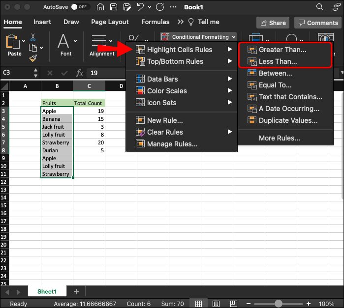
3. Navigate to “Highlight Cells Rules” and select the “Greater Than” or “Less Than” depending on the values you’d like to highlight.
   
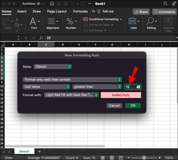
4. Enter a number that’s great than or less than the values you’d like to highlight depending on the rule you selected in step 4.
   
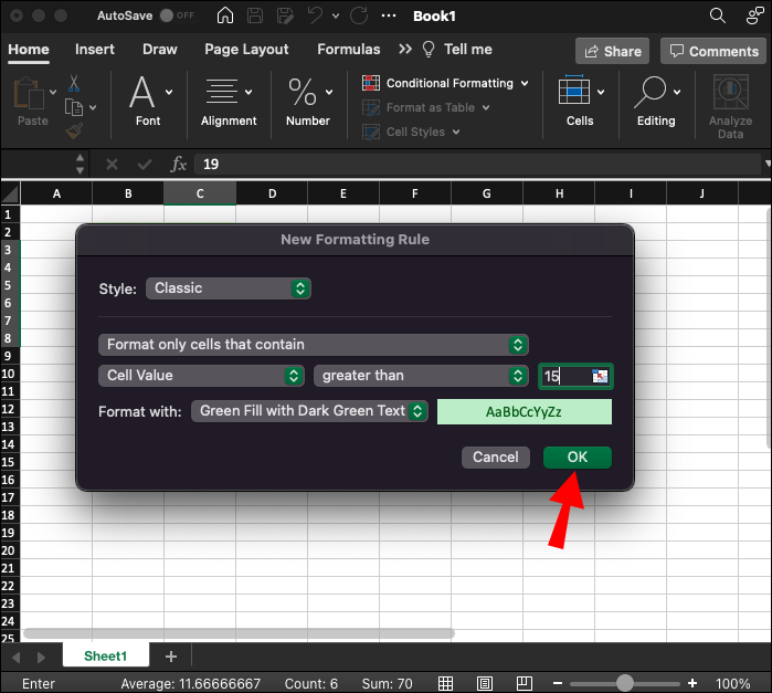
5. From the style presets on the right of the modal, select the style you’d like to apply to the highlighted cells.
   
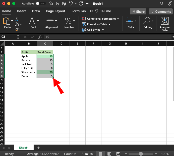
6. Click “OK” to save the changes.
   

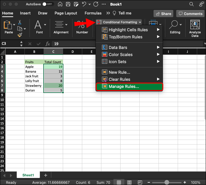
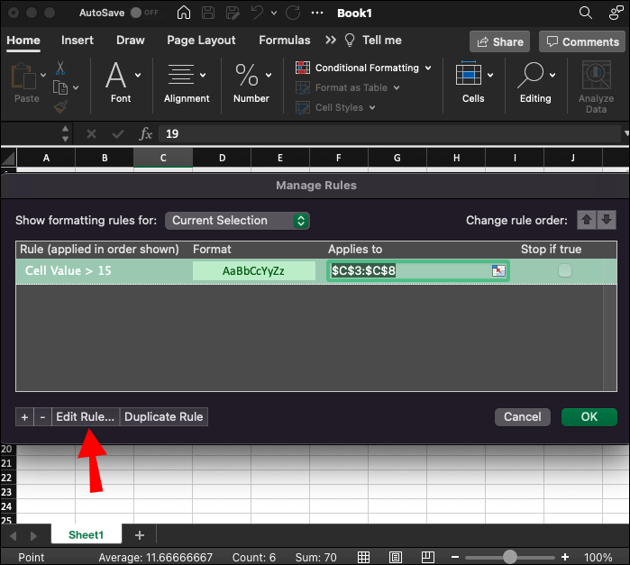
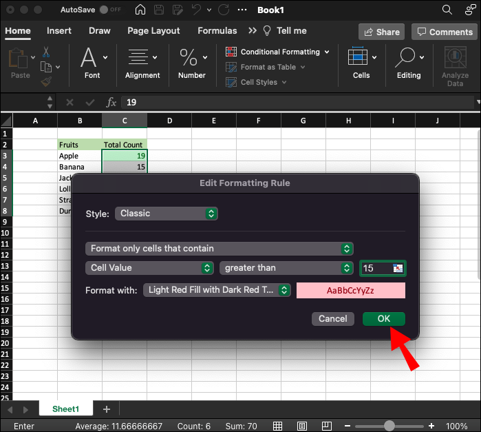
If you made a mistake while creating a rule, or maybe you just want to tweak it a little, you can easily alter it using these steps:

1. Select the cells whose rules you want to change.
   
2. Under “Home,” navigate to “Conditional Formatting” then “Manage Rules.”
   
3. Select “Edit Rule” and replace the preexisting value with a new value.
   
4. Click on the “Format” button to change the style of the highlighted cells.
   
5. Click “OK” to save the changes you’ve just made to the rule.
   

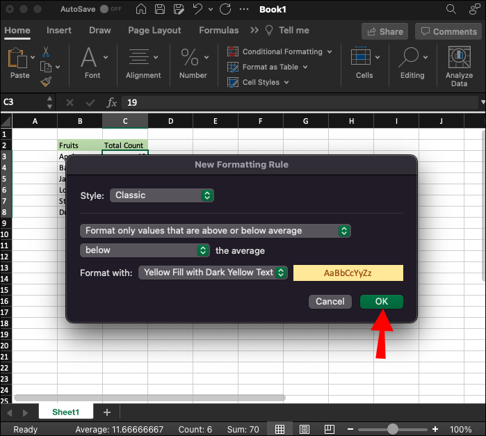
How to Highlight Values That Are Above or Below the Average in Microsoft Excel

Here’s how to highlight values that are less than a specific value in your Excel sheet:

1. Open the Excel sheet you need. Select the row, column, or the range of cells you want to work on.
   
2. On the ribbon menu, click on “Conditional Formatting.”
   
3. Go to “Top/Bottom Rules” then “Above Average” or “Below Average,” depending on what you need.
   
4. Select the style you’d like to apply to the highlighted cells from the dropdown options on the right of the modal.
   
5. Click “OK” to save the changes.
   

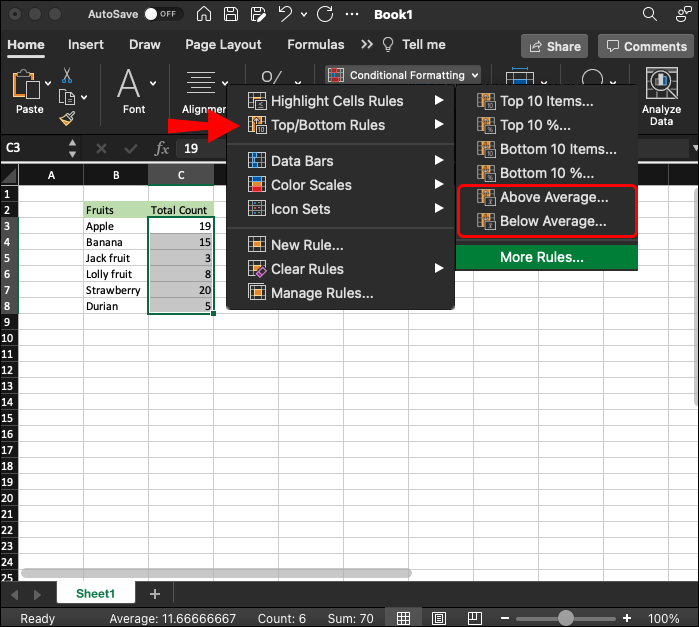
The “Top/Bottom Rules” section can also work with specific number of items or a percentage. For example, you can highlight only the top 10 values by using the “Top 10 Items…” selection.

How to Highlight Values That Are Greater Than a Specific Number in Microsoft Excel Using a Formula

While the built-in “Greater Than” and “Less Than” rules make the process a snap, using a formula gives you greater flexibility and control over the spreadsheet you’re working on. Plus, formulas are just a great way to get your creative juices flowing. Here’s how to use a formula to highlight values that are greater or less than a user-specific value in Excel

1. Select the column whose values you want to highlight.
   
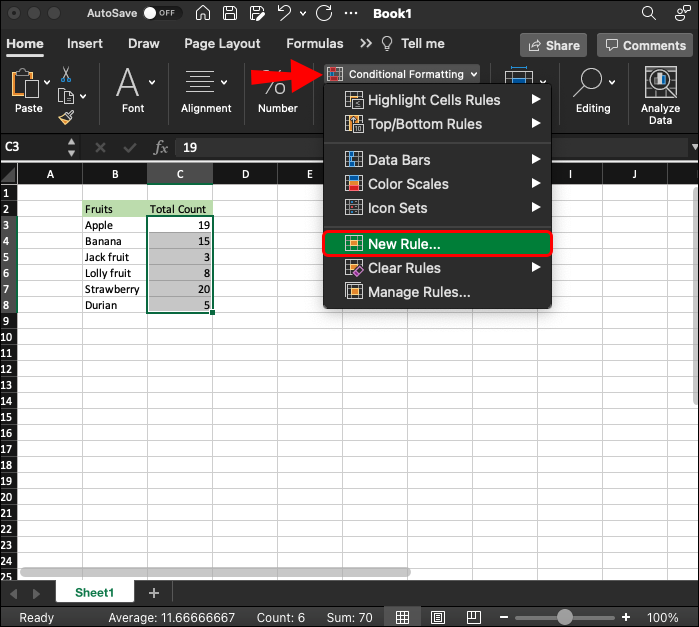
2. Navigate to “Conditional Formatting” then “New rule.”
   
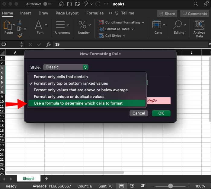
3. From the rule types, select “Use a formula to determine which cells to format.”
   
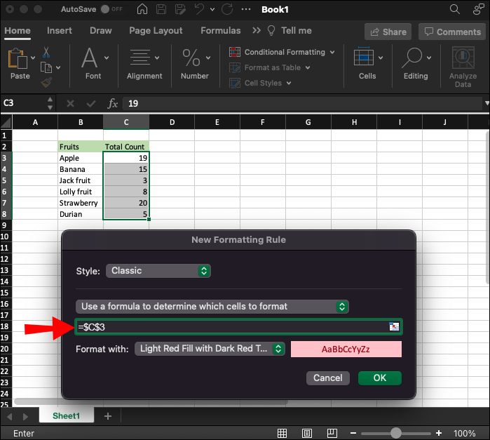
4. Click on the first cell of the column to automatically generate its address onto the formula box. (Feel free to drag the formula modal aside to get more room for the sheet you’re working on)
   
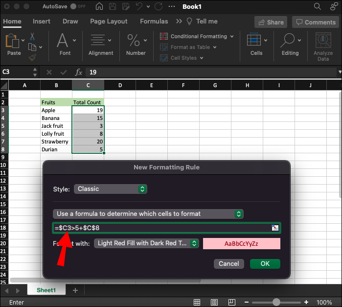
5. Next to the generated address, type in the “>” symbol followed by a number that’s less than the values you wish to highlight. If you wish to highlight values that are greater than a certain number, use the “<” symbol, followed by a number that’s greater than the values you wish to highlight instead.
   
6. Remove the second “$” symbol from the formula. If the symbol is not removed, the entire column will be highlighted rather than the cells that meet the predefined condition. The final formula should be something like this: =$A1>20+$A$5.
   
7. Click the “Format” button and select “Fill” and choose a color of your preference.
   

How to Highlight Words That Are Great or Less Than a Specific Alphabet in Microsoft Excel

It’s tempting to think that greater and less than rules only apply to numerical values, but that’s far from the truth. For instance, if you have a column of words and would like to highlight the ones that occur before or after a certain letter (or another word), you can easily do so using conditional formatting. Essentially, words greater than the benchmark word would appear later in a dictionary, and vice versa. Here’s how you do it:

1. Select the cells containing the words you’d like to highlight.
   
2. Navigate to “Home” then “Conditional Formatting.”
   
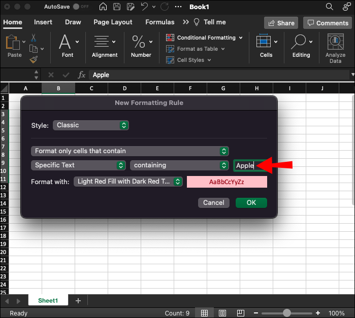
3. Go to “Highlight Cells Rules” and from the menu, select “Less Than” or “Greater Than” depending on what you aim to accomplish.
   
4. Input the letter or word that you want to compare against.
   

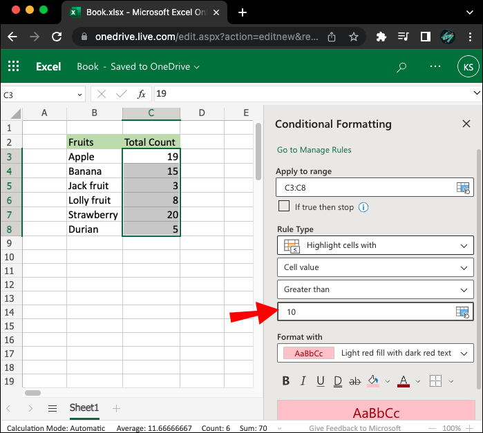
How to Highlight Greater or Less Than Values in Microsoft Excel Online

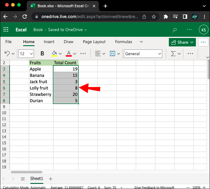
Excel Online is a web-based version of the desktop app. The web-based solution is useful if you like having a copy of your spreadsheet backed up on the internet. That way, your documents aren’t susceptible to system failures or hardware malfunctions which are common while working on a local workstation. Here’s how to highlight values that are greater or less than using the online app:

1. Open Excel Online.
   
2. Create or open the spreadsheet whose values you’d like to highlight.
   
3. Select “Home” and click on the downward arrow on the left to switch to the ribbon menu.
   
4. Select the columns whose values you want to highlight and click on “Conditional Formatting.”
   
5. Navigate to “Highlight Cells Rules” and choose “Greater Than” or “Less Than” depending on what you wish to accomplish with your spreadsheet.
   
6. Enter a number less or more than the values you’d like to highlight, depending on what you’ve chosen in step 5.
   
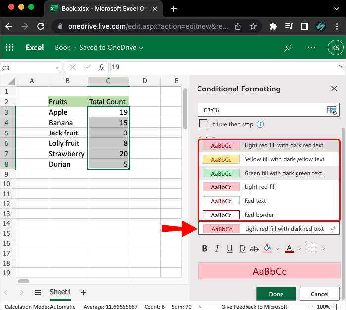
7. From the “Format with” dropdown menu, select a style you’d like to apply to the highlighted cells from the presets provided. If you want a custom format, select “Customized Format” from the menu.
   
8. Scroll down the modal and click on “Done” to persist the changes.
   

Additional FAQs

Can you highlight great or less than values using the Microsoft Excel mobile app?

Microsoft Excel mobile app is great for viewing and inserting data into your spreadsheets. However, highlighting values using the app can be challenging because it doesn’t support conditional formatting.

Can you use more than one rule on a single column in Excel?

Yes, you can add as many rules to a single column as possible. To do so, just select the column and add another rule.

Start Highlighting Like a Pro

Highlighting values that are great or less than throughout your Excel sheet is an excellent way to keep organized and on top of crucial patterns and trends. Fortunately, doing so is extremely simple because Excel includes built-in rules that automate the entire process. Plus, if you’re good with numbers, you can opt for a formula instead. Whatever your taste, we hope you can now highlight cells that are greater than or less than a certain value in Excel.

Have you tried highlighting values that are greater or less than a specific value in your Excel sheet? Did you use a custom formula or the built-in Excel rule? Please let us know in the comments section below.