How to Name Columns in Google Sheets

As you may have noted, columns in Google Sheets already have their default headers. We’re talking about the first cell in each column that will always be visible, no matter how much you scroll down. That’s very convenient, right? However, there’s one problem. Their default names range from A to Z, and there’s no way to change them.

But don’t worry. There’s another trick you can use to name columns in Google Sheets. In this article, we’ll explain how to name them the way you want and make everything more convenient.

How to Name Columns in Google Sheets

You always see A-Z columns because they’re frozen; they don’t disappear even when you scroll down and all other cells disappear. You can’t change their names, but you can freeze cells from another row and give them any name you want. That’s the way to change the default column headers and add your own names.

If you’re using Google Sheets in your browser, here’s what you have to do:

1. Open the sheet that you want to edit.
   
   
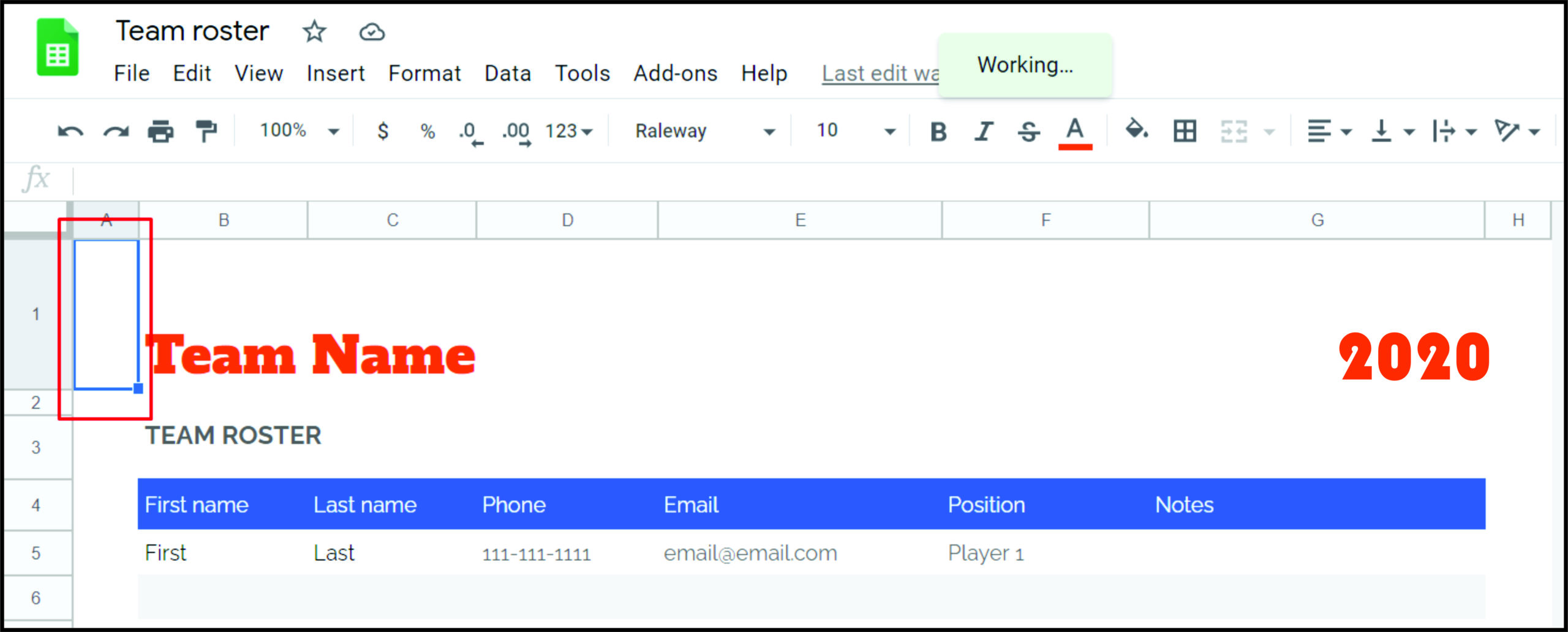
2. Click on the number in front of the first row.
   
   
3. Click on “Insert.” and select “Row above.” You should now get a new, blank row on the top of the document.
   
   
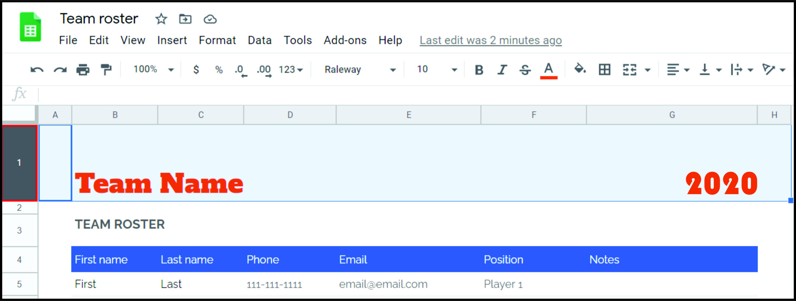
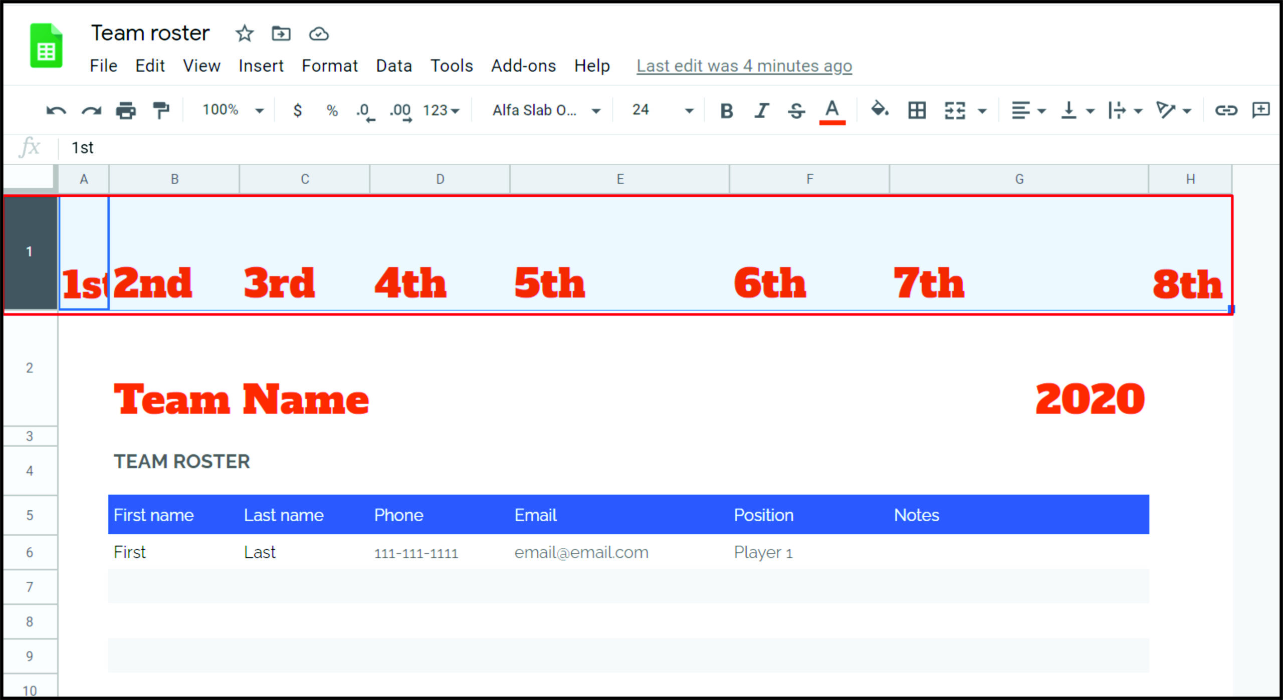
4. Enter the name of each column in the cells of the first row.
   
   
5. To highlight this row, click on the number in front of it.
   
   
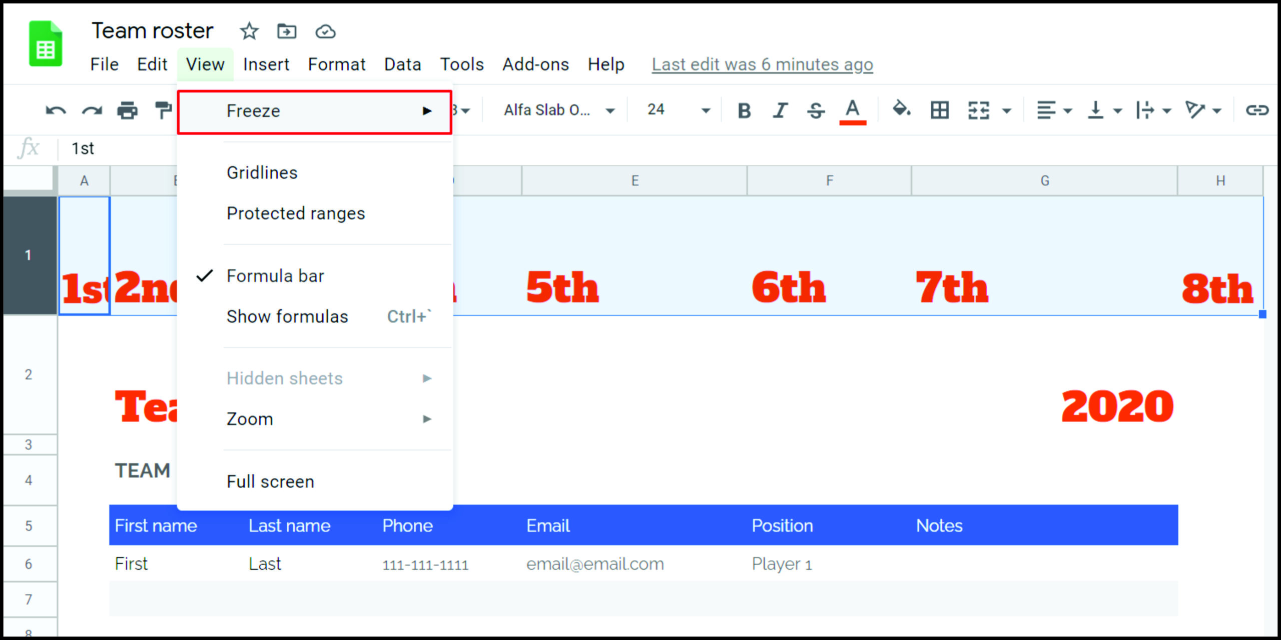
6. Click on “View.”
   
   
7. Select “Freeze.”
   
   
8. When the “Freeze” menu opens, select “1 row.”
   
   

There you have it. The row with column names is now frozen, which means you can scroll down as much as you want, but you’ll still be able to see your column names at the top. They’re your new headers, actually.

You can also sort and filter data by simply clicking on the column header. However, you first need to enable this feature. Here’s how:

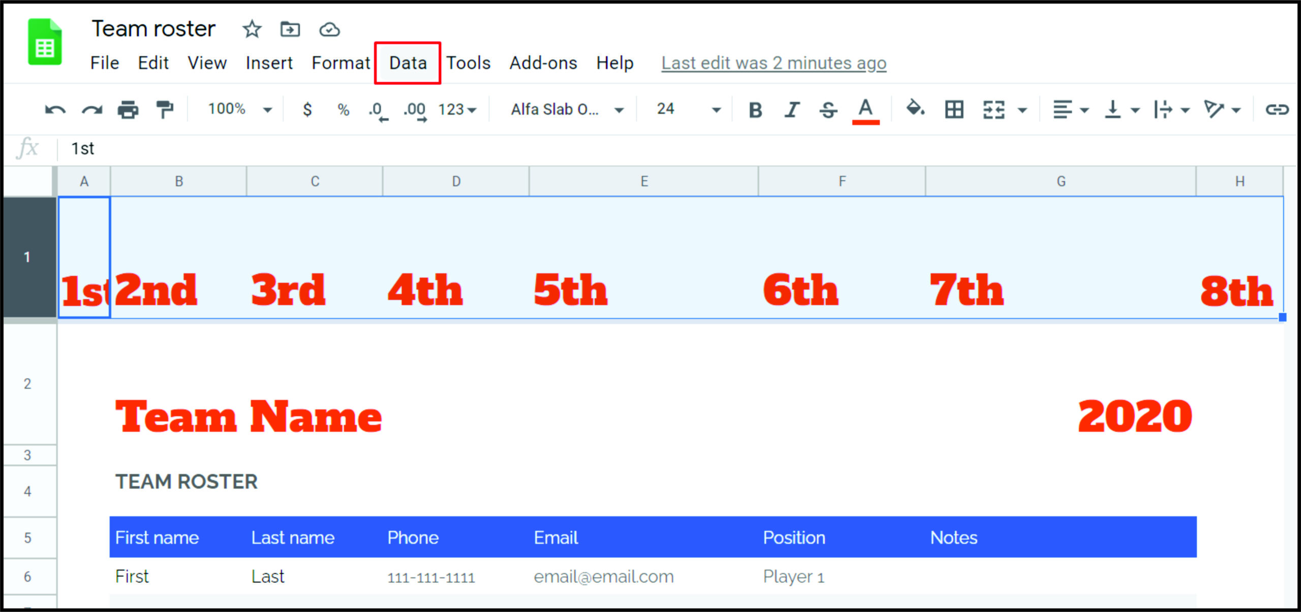
1. Go to the top menu and click on “Data.”
   
   
2. Select “Filter” and turn it on.
   
   

You’ll see the green icon in each header, and you can simply click on it to sort and filter data.

How to Name Columns in Google Sheets on iPhone

You can name columns using your iPhone as well, but you need to have the Google Sheets app. It’s not possible to do it from the mobile phone browser. Download the app, and we’ll show you how to name columns by changing headers and freezing them. The process is similar to what you do on your computer, but the steps are a bit different.

Here’s what you have to do:

1. Open the Google Sheets app.
   
   
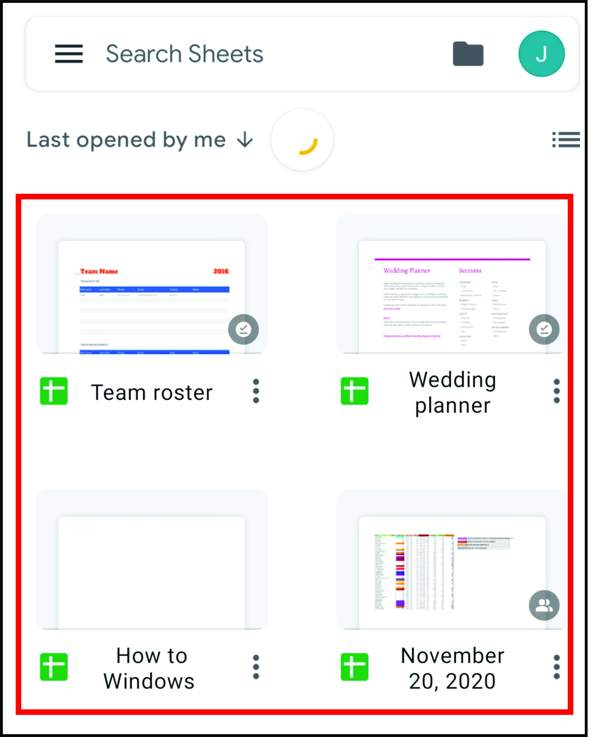
2. Open your spreadsheet.
   
   
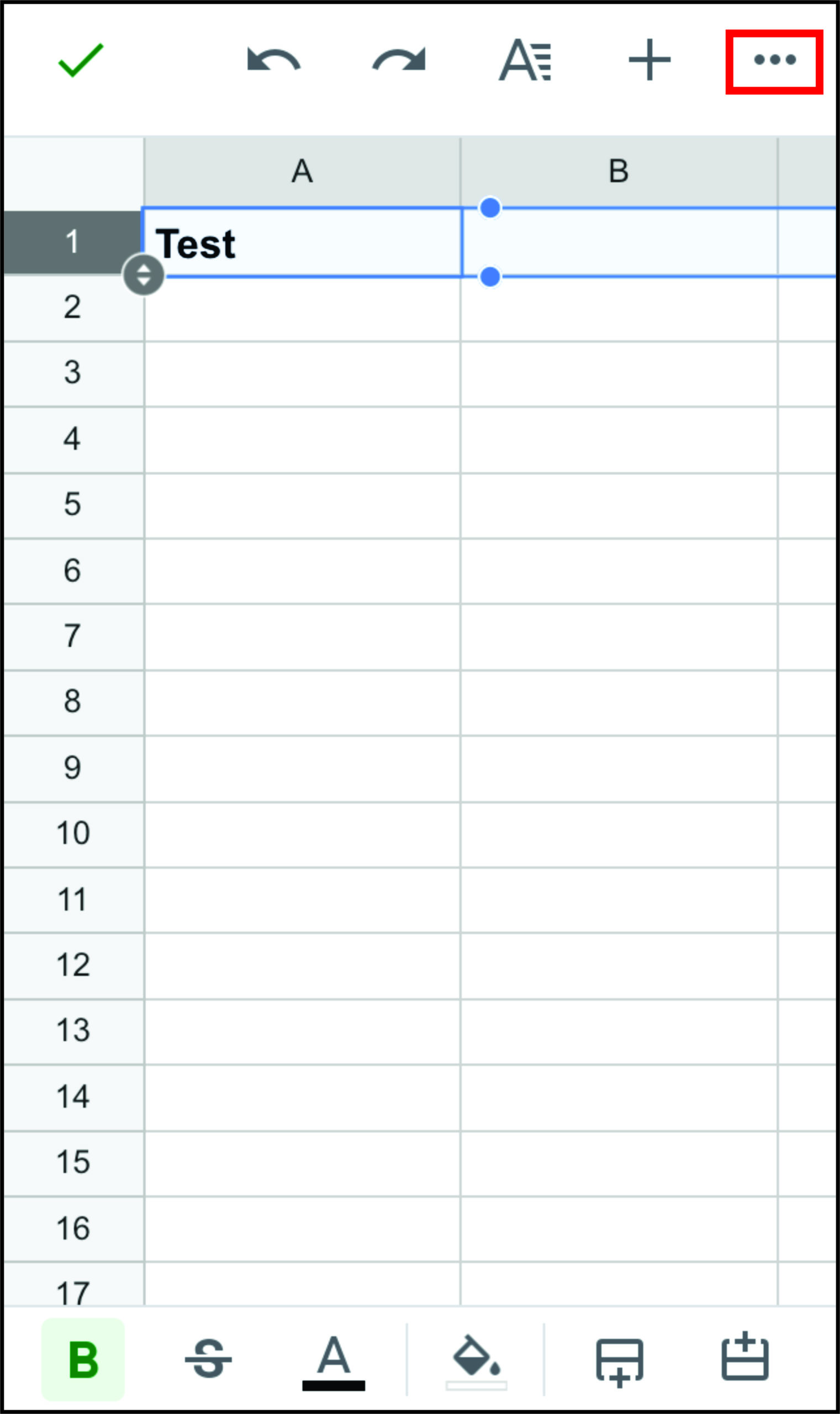
3. Tap and hold the first row.
   
   
4. When the menu appears, tap on three dots to see more options and select “Freeze.”
   
   

Freezing rows in the iPhone app is even easier than on a computer, as you’ll see a gray line dividing the frozen row from the rest of the document. It means you did everything correctly. That’s your new header. Now, simply enter the name of each column. When you scroll down, you’ll notice that the title doesn’t move, so you’ll always be able to see the column names. So convenient!

How to Name Columns in Google Sheets on Android

If you have an Android phone, there are two ways to name columns. While the first way is similar to the iPhone’s process, the second is a bit different. It consists of naming a range of cells. We’ll show you both ways so you can decide which one is more convenient for you. Before we start, make sure to download the Google Sheets app for Android.

Here’s the first method:

1. Open the app.
   
   
2. Open your spreadsheet.
   
   
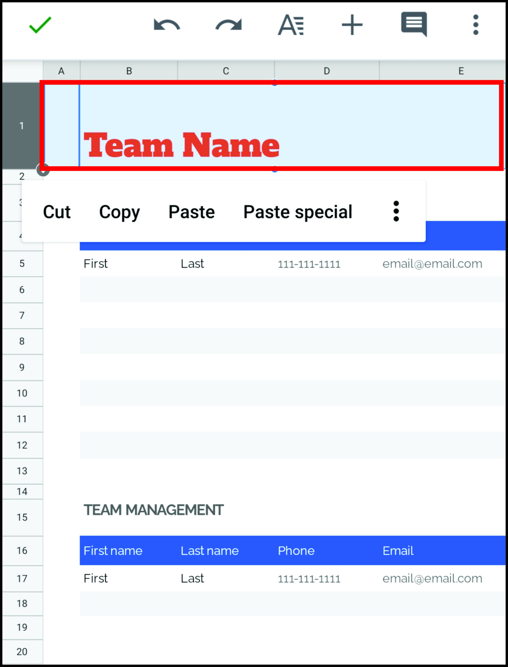
3. Tap and hold the number in front of the first row. This should highlight the whole row and open a toolbar.
   
   
4. Click on the three dots sign in the toolbar.
   
   
5. Select “Freeze.”
   
   
6. Double-tap a cell in the first row.
   
   
7. Enter the column name.
   
   
8. Tap on the blue checkmark to save.
   
   
9. Repeat the process for the first cell in each column.
   

There you have it You’ve just created headers with column names that are frozen and won’t move even if you scroll to the end of the document. However, if you’d like to try another method as well, here’s what you have to do:

1. Open the app.
   
   
2. Open your spreadsheet.
   
   
3. Tap on the three dots to get more options.
   
   
4. Select “Named ranges.”
   
   
5. Tap a named range to see it in your sheet.
   
   

Unfortunately, you can’t edit named ranges in the Google Sheets app. To do so, you may need to open the spreadsheet on your computer.

How to Name Columns in Google Sheets on iPad

Naming columns using your iPad is very similar to naming columns using your iPhone. Of course, everything may depend on the model you’ve got, but the process is generally similar. Download the Google Sheets app for the iPod, and let’s get started. Here’s what you have to do:

1. Open the app.
2. Open your spreadsheet.
3. Tap and hold the first row to highlight it.
4. You’ll now see a menu. Depending on your iPad model, you should tap on “More options” or the three-dot sign.
5. Choose “Freeze.”
6. Select “1 row.”
7. Now, double-tap each cell in the first row and enter the names.

There you have it. You’ve just created a custom header with column names that will always stay on the top of your document. The best thing is that Google Sheets automatically syncs, so when you open the spreadsheet on your iPhone or Mac, you’ll still be able to see the headers you’ve created.

How to Name Cells in Google Sheets

We’ve explained everything about naming columns, but what if you simply want to name a range of cells? There’s an easy way to do it, and we’ll explain everything you need to know. This can be very helpful, especially if you’re dealing with a lot of formulas. Instead of typing “A1:B10” every time, you can simply type your custom name, such as “budget” or “expenses.”

Here’s how to name cells in Google Sheets:

1. Open your spreadsheet.
   
   
2. Select all the cells you want to name.
   
   
3. Click on “Data.”
   
   
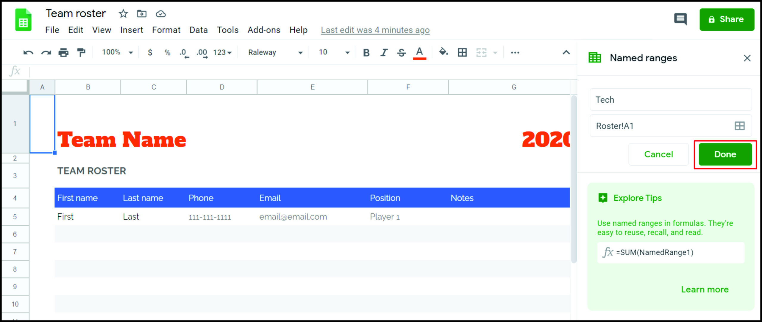
4. Select “Named ranges.”
   
   
5. Enter the name you want to use.
   
   
6. Click on “Done.”
   
   

That’s it. If you want to name more cells, simply select another range of cells in your spreadsheet. If the field is too large to select with your mouse, you can choose it by typing the cell range in the text box.

Bear in mind that the name can’t contain any spaces or punctuation. Also, it can’t start with a number, although it can include numbers.

How to Change Column Names in Google Sheets

The most challenging part is to name columns and create new headers. Once you’ve done so, changing column names will be effortless for you. Here’s what you have to do:

1. Open your spreadsheet.
   
   
2. Click on the cell in the first row containing the column name.
   
   
3. Go to the text bar, erase the old name, and enter the new name.
   
   
4. Press “Enter” to save.
   
   

There you have it. No matter what you rename it, this cell should stay your header. However, Google Sheets sometimes has trouble with some headers, and it may change your settings. But there’s nothing to worry about and if this happens, all you have to do is freeze that row again.

Additional FAQs

How to Alphabetize Google Sheets Columns

If you want to sort the columns alphabetically, first select all the columns you want to alphabetize. Then, open the top menu and click on “Data.” Click on “Sort sheet by A to Z.” Alternatively, you can also select “Sort sheets by Z to A” if you want to alphabetize them the other way around.

If you want to keep your headers and sort all other cells, make sure to select the “Data has header row” option. That way, Google Sheets will exclude your titles from sorting and treat them as a separate row, just like they should be.

How Do I Make a Column Header in Google Sheets?

Making custom headers in Google Sheets is very easy. All you have to do is add a blank row to the top of your document. Enter the name of each header and then freeze that row. If you’re using the Google Sheets app, you’ll see a gray line that’s now separating the column header from the rest of the cells.

The cells in the frozen row will function as column headers as they will stay on the top. You’ll always be able to see them, even if you scroll to the bottom of the document. You can also exclude your headers from formatting and format all other cells in your spreadsheet.

Customize

Many people aren’t particularly fond of the default column names in Google Sheets. They aren’t very helpful when you’re dealing with a lot of data, and letters A-Z probably won’t be useful to you. Thankfully, there’s a way to name columns the way you want and to make the names stick. We hope that this article was useful to you and that you’ve learned something new.

Do you customize columns and rows in Google Sheets? Is there any other trick that helps you organize your columns? Let us know in the comments section below.