At its core, Excel appears pretty basic. The more you get into it, however, the more you realize it’s not all about making tables – it’s actually about creating spreadsheets.
Often, you’ll work with more than one Excel spreadsheet. You may, for example, have to compare sheets to see if there are any differences. In this respect, Excel allows you to do to just that. This can be of tremendous importance. Here’s how to check whether two spreadsheets are identical.
Comparing Two Sheets
Let’s assume that you’re trying to compare two sheets within a workbook. You’ll probably want the side-by-side view.
To gain this view, navigate to the View tab in Excel, located in the upper part of the screen. Then, click Window group. Now, go to New Window.
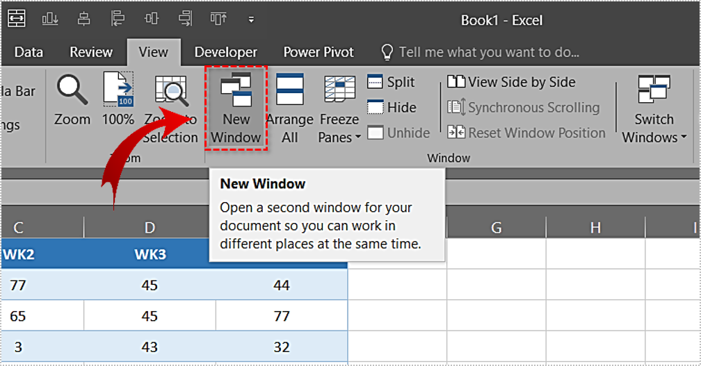
This command will open that Excel file, only in another window. Now, find View Side by Side and click it.

Finally, navigate to the first sheet in one window and the second sheet in the other.


Comparing Two Excel Sheets
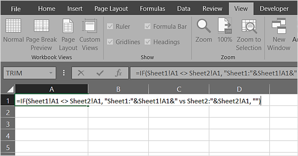
The best way to see if two Excel sheets are an exact match would be to check for differences in values. If no differences are found, they’re identical.

Now that you have the two sheets that you want to compare side by side, open a new sheet. Here’s what to enter in the cell A1 in the new sheet: “=IF(Sheet1!A1 <> Sheet2!A1, “Sheet1:”&Sheet1!A1&” vs Sheet2:”&Sheet2!A1, “”)”
Now, copy this formula down and to the right using the Fill handle (a small square at the bottom-right cell corner).
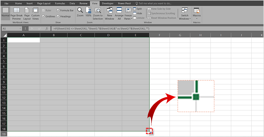
This will mark all the differences in cells in the two sheets that you’re comparing. If there are no differences displayed, that means that the worksheets are perfect matches.

Highlighting the Differences
Sometimes, you’ll want to mark the differences between two worksheets. You may want to make a presentation, or simply mark it for yourself. Whatever the reason, here’s how to highlight the differences.
For the purposes of this article, we’re using Excel’s conditional formatting feature. Choose a worksheet where you want to highlight the differences. In it, Select all used cells. Instead of dragging the selection, select the upper-left cell and then press Ctrl + Shift + End. Now, with all the used cells selected, go to the Home tab, navigate to Styles, and select Conditional Formatting. Then, click New rule, and use this formula for the rule: “=A1<>Sheet2!A1”

Of course, “Sheet 2” in this formula is a placeholder for the actual name of the sheet that you want to compare.
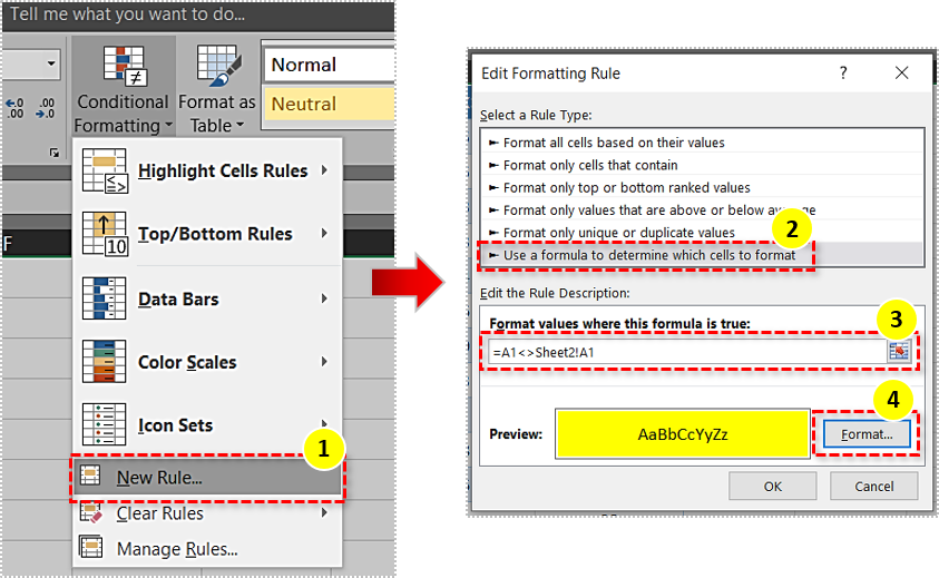
When you’ve entered the formula and confirmed, all the cells that have different values will be highlighted with the color that you’ve previously selected.

Comparing Two Excel Workbooks
It might seem like a lot of work, but you can actually compare two Excel workbooks pretty easily. Well, if you know how to use Excel, that is.
To compare two workbooks, open the two that you want to compare. Then, navigate to the View tab, go to Window, and select View Side by Side.
The two workbook files will be displayed side-by-side, horizontally. If you prefer seeing them as a vertical split, navigate to the Arrange All function under the View tab and select Vertical.

Here’s a cool tip about comparing workbooks in Excel. Navigate to the View Side by Side button, but don’t click it. Right under it, you’ll see the Synchronous Scrolling function. Click it instead. This will allow you to scroll the two workbooks that you’re comparing simultaneously. Pretty neat!

Checking Whether Two Excel Sheets Are a Match
You don’t have to be a coder to successfully compare two Excel sheets. All you need is some basic Excel experience and practice. If you’ve never compared two sheets or workbooks before, dedicate some time to it, as it will take a little while to get used to.
Have you managed to compare two Excel sheets? What about two workbooks? Did you find anything unclear? Feel free to drop a comment below with any questions, tips, or remarks about comparing sheets and workbooks in Excel.
Disclaimer: Some pages on this site may include an affiliate link. This does not effect our editorial in any way.