How to Find Duplicate Rows in Excel

Perhaps you’re working with a lot of information in Excel. Duplicate rows don’t make the process easier. You’ll want to eliminate them to make your database readable, neat, and orderly. However, before deleting them, you’ll need to find them first. Fortunately, a few methods and functions automatically identify these rows for you.

Read on to learn how to find duplicate rows in Excel.

How to Locate Duplicate Rows on Excel Using the COUNTIFS Formula

You’ll need to use the COUNTIFS formula in Excel’s formatting option to identify and highlight your duplicate rows. Here’s how to do so:

1. Select your desired range where you want to check for duplicate rows. If it’s the whole workbook, then use the command CTRL + A.
   
2. Navigate to the home tab and select the “conditional formatting” option in the styles group. It’s the grid icon with blue, white, and red squares.
   
3. Select the “new rule” option and “use a formula to determine which cells to format.”
   
4. Add the formula COUNTIFS($A$2:$A$100, $A2, $B2:B$100, $B2)>1 in the box and choose a formatting style.
   
5. Select “Ok.”
   

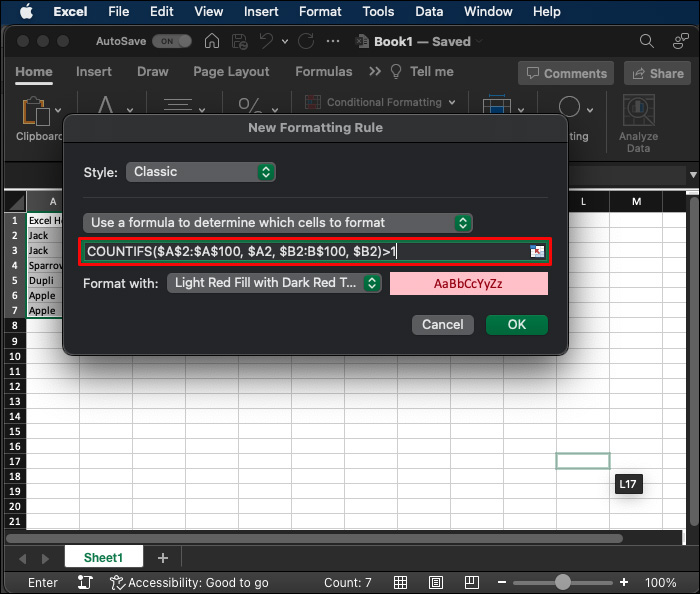
However, keep in mind that the formula assumes that the data starts at A2 and ends at B100. You need to change the function depending on your specific range, and append arguments for any additional column (such as “, $C$2:$C$100, $C2“) to the COUNTIFS formula.

Excel will automatically highlight all the duplicate rows within your entire selected range.

If this doesn’t work, copy the formula to a helper column for each row and format it according to that cell’s output.

Highlighting Duplicate Values in Excel

This is the most straightforward way to identify duplicate values in your workbook. You won’t have to use complicated functions, just the home tab. Here’s how to do it:

1. Select the whole range in which you want to check for duplicate rows.
   
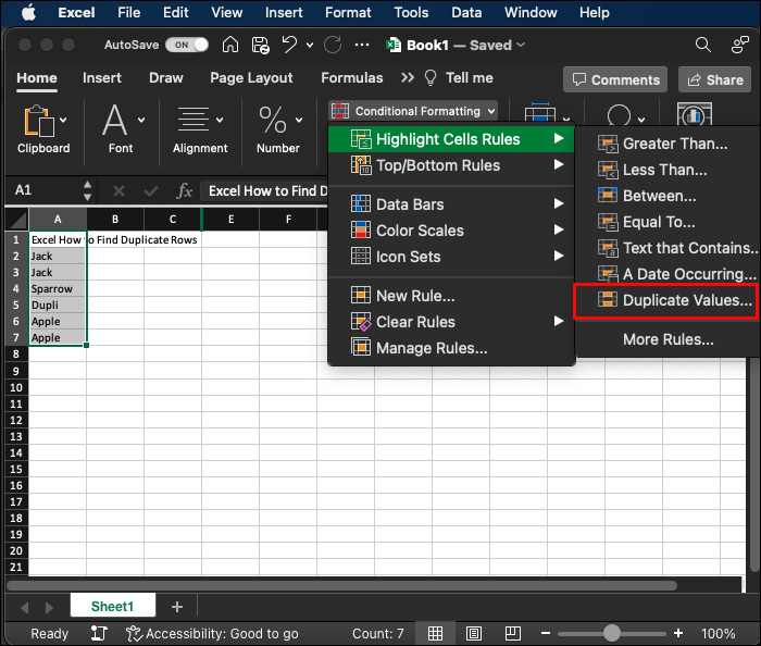
2. Go to the home tab and select the “Conditional Formatting” option in the styles group. The icon shows a grid with red, white, and blue squares.
   
3. In the open tab, select “Highlight cell rules” then select the “Duplicate Values” option.
   
4. Select your desired formatting style in the window that pops up and click on “Ok.”
   

Excel will then highlight any duplicate values within your selected cells. You can even change the highlighting color within the formatting pop-up menu when it appears.

This is an imperfect method since it identifies duplicate values rather than entire rows. It can produce inaccurate results if a row contains cells that are duplicated across columns.

However, it can be much easier to implement and see in smaller spreadsheets.

Highlighting Triplicate Values in Excel

If you want to clean up your workbook, you can also identify triplicate values. The process requires making a new rule rather than using Excel’s default formatting options. Here’s how to do it:

1. Select your desired range of values where you want to check for triplicates.
   
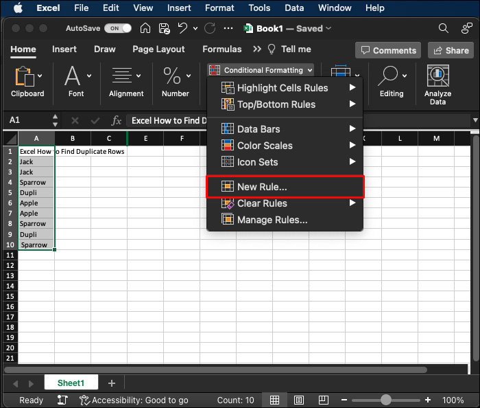
2. Go to the home tab and select the “Conditional Formatting” option in the Styles group.
   
3. Select the “New Rule” option.
   
4. Click on the “Use a formula to determine which cells to format.”
   
5. Use this formula: =COUNTIFS($A$2:$A$100, A2, $B2:B$100, B2)=3. Using this formula checks if the row appears three times within your chosen range. This once again assumes you’re using a range from A2 to B100.
   

It’s as simple as that! Excel will identify and highlight triple values within your selected range. However, keep in mind that the formula above identifies triple values for the cell you set (identified in function as (($A$2).

You can simplify the formula with COUNTIF($A$2:$B$10, A2) instead. This only checks for the contents of the current cell within the range, so will highlight cells across rows and columns.

Deleting Duplicates and Triplicates in Excel

Perhaps you’ve highlighted all the duplicates or triplicates in your workbook using the above method. Afterward, you may want to delete them. This will make your whole workbook neater and less confusing.

Fortunately, deleting duplicates once highlighted is a simple task.

Here’s how to do it:

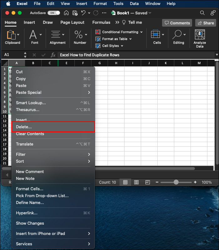
1. Select the highlighted rows by clicking the row numbers while holding down CTRL (Command in Mac). This will make Excel select all the highlighted rows.
   
2. Hover over one of the selected row numbers, right-click and select the “Delete” option.
   

Deleting rows might alter the overall formatting of your workbook. You should also consider recording the information on the deleted rows in case you need it later. There are also a few other ways to delete the highlighted duplicate and triplicate rows quickly:

1. Select the highlighted rows by clicking on their numbers while holding down the CTRL/Command key.
   
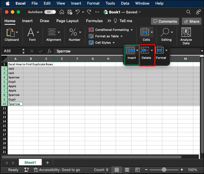
2. Navigate to “Home,” located at the upper Excel ribbon, in the “Cells” option,
   
3. Select “Delete Sheet rows.”
   

Another convenient way to delete rows is by using a command once you highlight them. Simply use the key shortcut “CTRL + -“,”Cmd + -.” This will delete all your selected rows (or values), and you’re good to go.

When to Highlight and Delete Duplicate and Triplicates in Excel

There are a few instances when highlighting duplicates and triplicates and deleting them will be useful for your workbook. Even if you don’t need it immediately, the methods above can be used for some of the following real-world examples:

• Database entry errors – You might accidentally enter the same information twice. With such mistakes, highlighting duplicates can be an easy way to identify and subsequently delete the errors.
• Database merging errors – Sometimes, you’ll need to combine multiple databases into one. During the merging process, additional errors can occur, resulting in duplicated rows.
• Email lists and customer database duplicates – Duplicates in customer databases can result in sending a customer marketing material such as the same newsletter twice. This can be annoying and deter customers from your service. Deleting these rows is the best course of action.
• Inventory management problems – Every product must be accounted for in warehouse inventory management environments. If duplicates and incorrect data are left in important databases, this can cause management discrepancies. Deleting rows in these instances leads to much more accurate tracking.

Other spreadsheets needing duplicate row identification include employee records, research, survey, and financial data. Deleting the extra rows will increase accuracy, time-saving when looking for relevant information, and easier data analysis.

Other Helpful Excel Methods You May Need

Duplicating rows is only one aspect of a wide range of useful Excel skills. You won’t need to spend hours studying them. They can be done with just a few simple key commands. For example, you might need to:

• Copy Rows – Simply select the rows you need and then use the command CTRL + C.
• Pasting rows- Once your rows are copied, you can go ahead and paste them by using the command CTRL + V. Alternatively, you can right click and select the option “Insert Copied Cells.”
• Delete certain cells – To get rid of certain cells, all you need to do is select them and use the command Ctrl + X to cut them and then clear the data.

These are all small but necessary commands you might need when dealing with duplicate rows within your workbook.

FAQS

Do I need to use formulas and functions to delete duplicate rows in Excel?

Yes, you’ll need to use the COUNTIFS function for this task. However, highlighting and deleting individual cells doesn’t require a formula or function.

Should I delete duplicate rows once I find them in Excel?

That depends on the purpose of your workbook. If it’s for maintaining inventory, duplicate rows can spoil the integrity and accuracy of the document. In such cases, it’s best to combine their data and remove the excess rows.

What if my workbook has lots of data?

You can easily select all the data in your spreadsheet, regardless of how much there is, by using the command CTRL+A. Once selected, you can continue with one of the methods for highlighting and deleting individual rows above.

Clean Up Your Data by Highlighting and Deleting Duplicates in Excel

Highlighting and deleting duplicates is a reasonably simple process for Excel users. You need to use the conditional formatting option for individual cells and the COUNTIFS or COUNTIF formula after entering the “new rule” option. After all your duplicates and triplicates are highlighted, you can delete them using the “delete sheet rows” option in the upper Excel ribbon or the “CTRL + -” command. Knowing how to highlight and delete duplicates is beneficial for multiple real-world scenarios, including inventory checks and managing database errors.

Did you find it easy to highlight duplicate rows in Excel? Which method did you use? Let us know in the comment section below.