How to Lock Cells in Excel

Lee Stanton August 29, 2023

One of the most impressive features of Microsoft Excel is that you can share your files with others for viewing/editing purposes. However, you sometimes don’t want them to tamper with the original data. Rather, you only need them to inspect the document and feed it back for revision without making any adjustments.

That’s where locking cells comes in, but how does it work? Here’s an in-depth guide on how to lock cells in Excel.

Locking Cells in Excel

Excel has been around for nearly four decades. Over the years, it’s undergone extensive changes, but some features have remained pretty much the same. One of which is locking cells.

The steps are similar, if not identical, in all versions of this spreadsheet program.

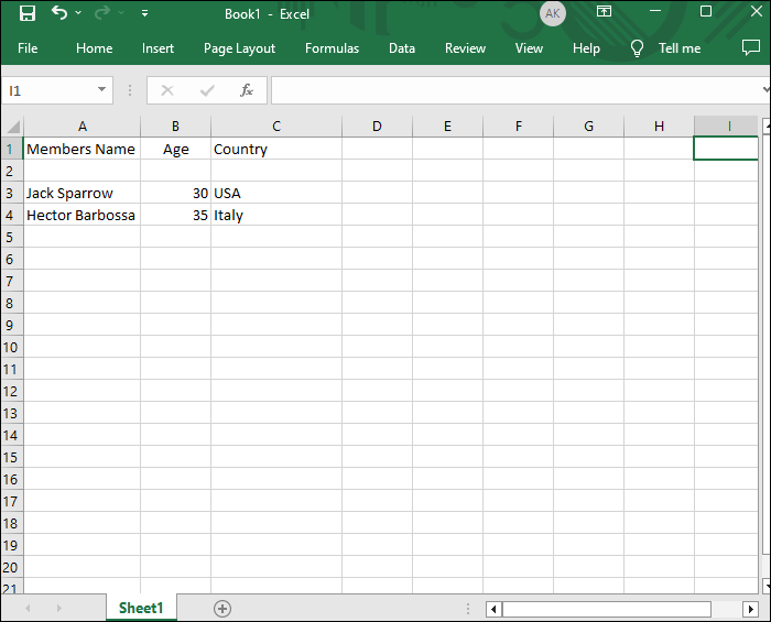
Open your spreadsheet.
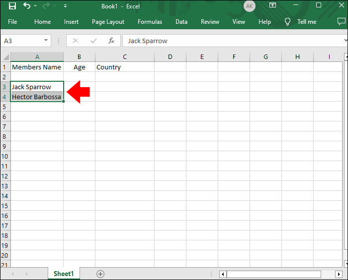
Highlight the cells you wish to protect. You can use your mouse or the “Ctrl + Space button” shortcut to do so.
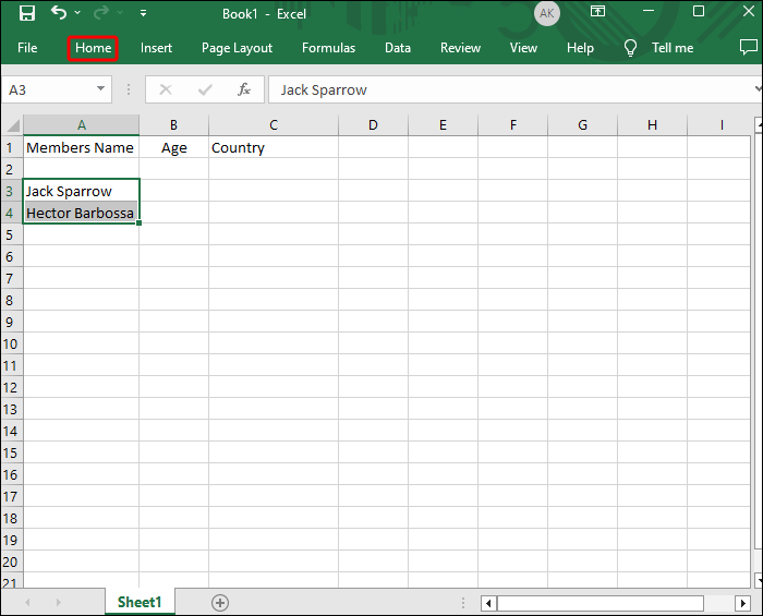
Navigate to your “Home” window.
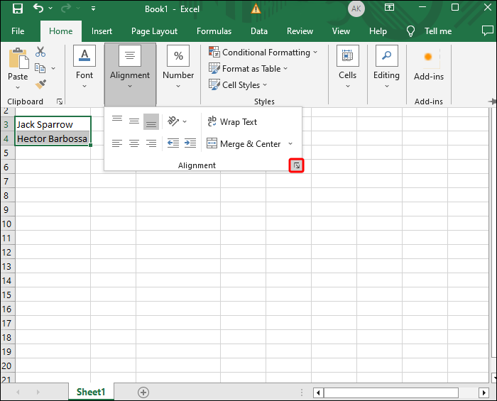
Choose “Alignment” and strike the arrow symbol.
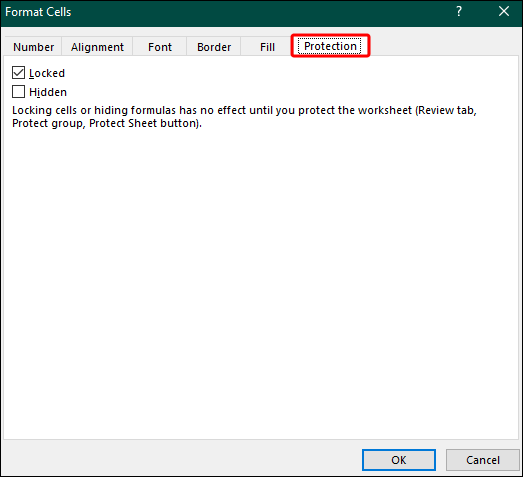
Head to your “Protection” menu.
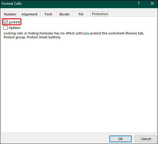
Pick “Locked.”
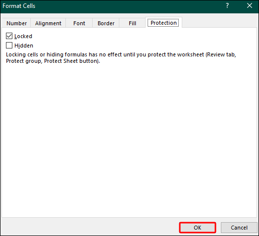
Strike the “OK” button to leave the menu.
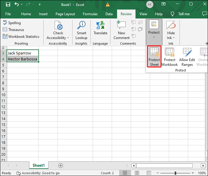
Access “Review,” go to “Changes,” select the “Protect Workbook” or “Protect Sheet” option and reapply the lock. Type in the password you’ll need to enter to unlock the cells.

That’s all there is to it. You’ll now be able to share your file without worrying about whether the other party will interfere with the data.

How Do You Lock All Cells in Excel?

The above steps enable you to lock specific cells in Excel. But what if you want to go one step further and lock all cells? That way, the user who you share the data with won’t be able to modify even the tiniest part of your worksheet. Plus, it eliminates the risk of leaving one or more cells unlocked accidentally.

It’s a comprehensive measure, but it’s just as simple as the first method.

Open Excel and find the spreadsheet you wish to lock.
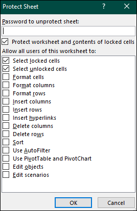
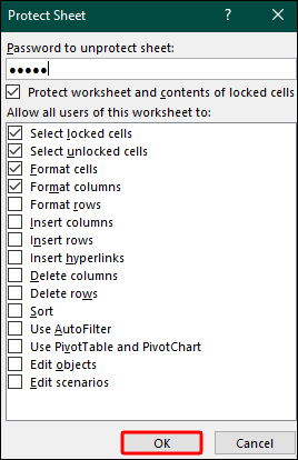
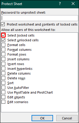
Choose “Review,” followed by “Changes,” and “Protect Sheet.”
You can now select a number of options to keep others from changing the cells, depending on your preferences:

a. “Locked” keeps the user from deleting or inserting columns and rows.
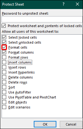
b. “Format Cells” keeps the user from enlarging or reducing columns and rows.
c. “Use PivotChart” and “Use PivotTable” keeps the user from accessing pivot charts and pivot tables, respectively
d. “Autofill” keeps the user from extending selected parts with the Autofill function.
e. “Insert and Delete” keeps the user from adding and removing cells.
Check the box next to the “Sheet” option.
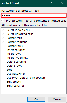
Enter the code the other party will need to use to unlock the cells if you decide to share the password with them.
Tap the “OK” button, and you’re good to go.

How Do You Lock Cells in Excel With a Condition?

A large part of working in Excel comes down to your ability to apply conditions. If you’ve made tremendous progress with your conditions and don’t want anyone to undermine it, locking your cells is a great option.

But this doesn’t mean you need to take sweeping action and lock all cells. Excel enables you to restrict only those with your condition.

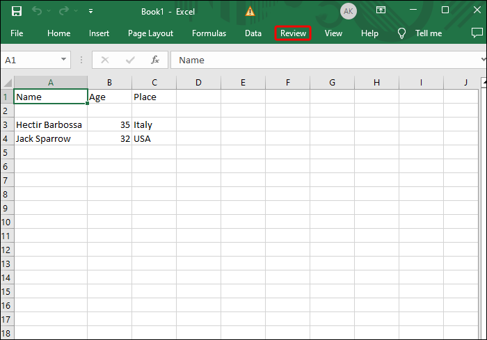
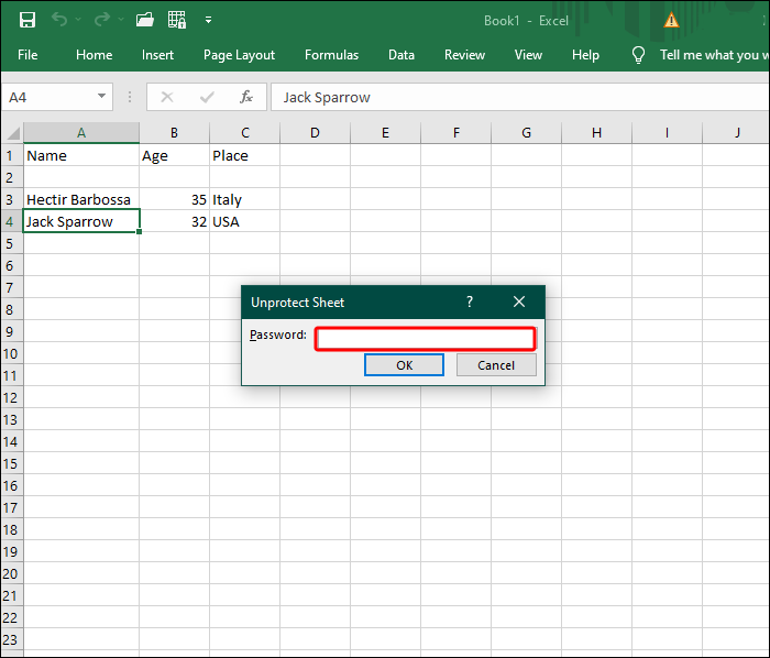
Bring up your spreadsheet and head to the “Review” section.
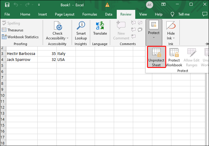
Navigate to “Changes” and click “Unprotect Sheet.”
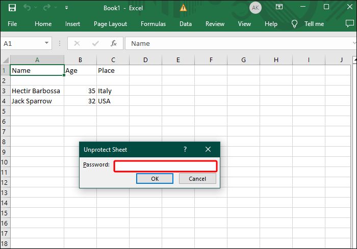
Enter the password you used to lock your sheet and tap the “OK” button. If you haven’t restricted your sheet, proceed to the next step.
Highlight the cells you wish to make off-limits with your mouse or the “Ctrl + Space” key combination.
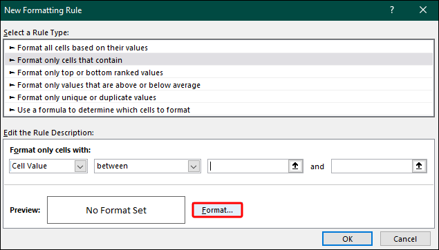
Apply “Conditional Formatting” and go to “Condition 1.”
Pick “Format” and select “Format Cells.”
Navigate “Protection,” check “Locked” next to the appropriate box, and choose “OK.”

How Do You Lock Cells in Excel Fast?

As previously discussed, the cell lock feature has been a staple of Excel for many years. It hasn’t undergone major overhauls, but it has been improved in recent versions. For example, more recent editions of Excel allow you to add a quick-lock button to your toolbar. It lets you restrict the highlighted cells with a single press of a button.

Let’s see how you can incorporate the function into your menu and how it works.

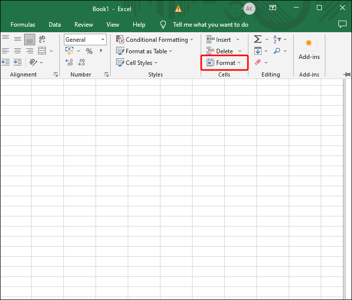
Open a spreadsheet and go to “Home.”
Find “Format” and select the “Lock Cell” feature.
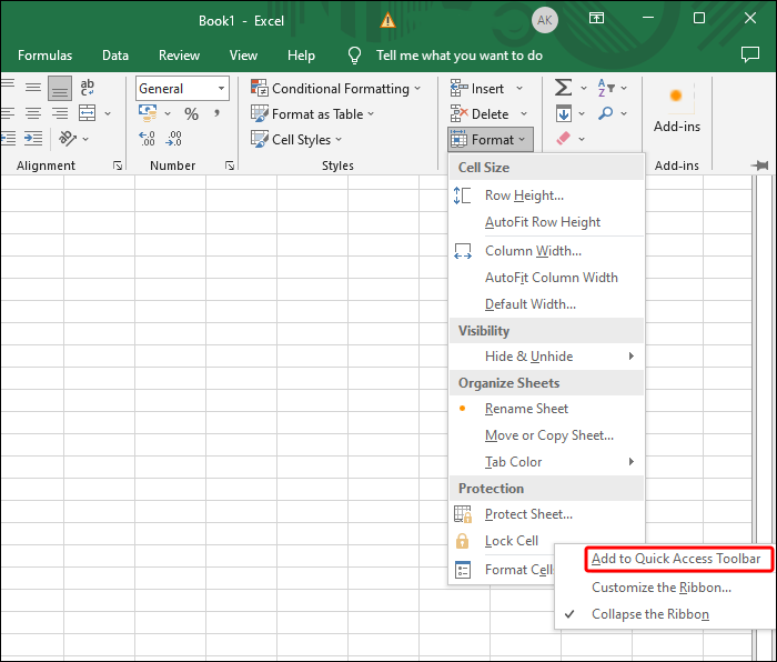
Right-click “Lock Cell” and choose the prompt that lets you include the function in your “Quick Access” section.
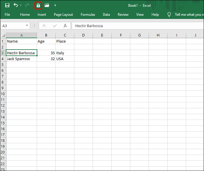
Head back to your spreadsheet and check out the lock cell shortcut in the upper part of your file.
To use the shortcut, simply select one or more cells and press the lock symbol in the toolbar. Depending on your version, the program may ask you to enter a password. You’ll know the cell is restricted if the shortcut key has a dark background.

How Do You Prevent Users From Selecting Locked Cells?

Keeping others from selecting locked cells is useful in two ways. First, it further reduces the risk of unwanted changes. And second, it helps boost the other party’s productivity by separating the available cells from the unavailable ones.

Start your spreadsheet and go to “Review.”
If your workbook is protected, press the “Unprotect Sheet” button in the “Changes” window.
Pick “Protect Sheet.”
Make sure the “Select locked cells” option is checked.
Tap “OK,” and you’ll no longer be able to highlight restricted cells. You can navigate between unlocked cells using your arrow keys, Enter, or Tab.

Shield Your Data From Prying Eyes

Although sharing data is inevitable when collaborating on an Excel project, there’s no reason to allow others to tamper with sensitive information. With the lock cell function at your beck and call, you can restrict as many cells as you want to prevent unauthorized changes.

Have you ever had data loss/data tampering issues in Excel? If so, what did you do to protect your data? Tell us in the comments section below.