You’ve created a gigantic spreadsheet in Excel and are having trouble finding certain values. Searching for the data manually would take too long, so is there a way to automate the process? There is – all you need to do is use a shortcut or function.
This guide will show you how to determine if a value is in a list using shortcuts and functions in Excel.
How to Look for Values in Excel With a Shortcut
While Excel can sometimes be complex, the tool keeps basic features simple. One of these easily accessible functions is the ability to look for values. The method is similar to how you’d achieve this in Microsoft Word, Notepad, and other programs. More specifically, you need to utilize the Find shortcut.
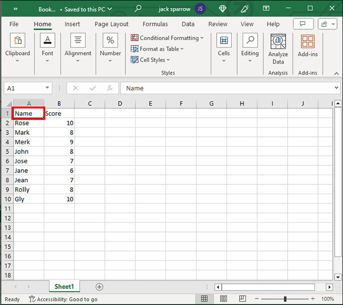
- Open the spreadsheet where you want to find your values.
- Choose the column or multiple columns that may contain the desired value.
- Strike the Ctrl + F key combination.
- Head to the Find window and type in the value you want to look up.
- Navigate to Find What, followed by Find All.

- If the tool retrieves matching results, it lists them in the window. If not, you’ll get a dialog box reflecting the failure.


If you want to search across the workbook or sheet, make sure no column is selected.
How to Look for Values in Excel Using Functions
On the other end of the spectrum are functions. They’re slightly trickier to apply than the shortcut feature, but many prefer them because they allow you to customize your search. Once you use a function, you can easily copy the formula down the sheet to apply to other cells.
You can utilize several functions to determine if your list contains a particular value.
MATCH and ISNUMBER
The first function we’ll consider is an embedded function. Here, the MATCH function is part of the ISNUMBER function. It might sound daunting, but it’s relatively easy to pull off.
In the Match function, the first number is the value you’re looking for. The second number is the list that may contain the value. The third number is 0, telling the function to look for identical values. The ISNUMBER function checks if the number if an actual number or something else.
- Open your spreadsheet.
- Click the cell where the function will tell you whether your list contains the value.
- Type in the following function: =ISNUMBER(MATCH).
- Here’s an example to give you a better idea: =ISNUMBER(MATCH D14, C5:C10,0), where D14 is the cell containing the value, and C5:C10 is the range where the tool will look for the value.
- Press Enter, and you’ll immediately know whether the value is in the list. If yes, you’ll get a True. If not, the function will provide a False in your originally selected cell.


COUNTIF
Another easy way to check for values in Excel lists is to utilize the COUNTIF function. This convenient feature can save the day even if you’re looking for a needle in a haystack.
COUNTIF is a simpler alternative; you only need to type in two parameters. First, tell the system where it should look for the value (the range). And second, tells the function what it’s looking for in inverted commas.
- Go to your spreadsheet.
- Highlight the cell where you’ll get the end result. In other words, this is where the function will tell you whether the value is in the list.
- Enter the following function in the cell: =COUNTIF
- Press Tab to launch the function and enter your values. Let’s use the same example here: =COUNTIF(C5:C10, “D14”)
- Press Enter to see whether the value exists in the list. If so, the function will also reveal how many instances of the said value appear in the data.


IF and COUNTIF
If the COUNTIF function doesn’t do the trick, no worries. The embedded version can be a lifesaver. You can add this function to the IF function for more logical expressions. This allows you to narrow down your search even further.
The COUNTIF Function will count the number of cells that meet a specific criterion. The function needs four parameters: the list, criteria (value), value if true, and value if false.
- Open your spreadsheet and press the desired output cell.
- Enter the following line in the cell: =IF(COUNTIF())
- Here’s an example: =IF(COUNTIF(C5:C10, “D14”), “Yes,”” No”). Here, you’re looking for data in cell D14 in the selected range. The function will give you a Yes in the highlighted cell if it exists. If not, you’ll get a No in the same cell.
- Press Enter, and you’re good to go.


How to Find the Highest Value in a List in Excel
As an Excel professional, you might be asked to retrieve the highest value in a particular list. The above functions will only get you so far if you don’t know the exact number.
The MAX function is your life jacket in such cases. As the name suggests, it extracts the maximum value from the selected list. You shouldn’t have trouble applying this formula.
- Select a cell.
- Type in =MAX()
- Select the list where the tool will look for the highest value. You can do so with your mouse.
- Enter the closing parenthesis and hit the Enter button to finalize the formula. For example, to find the maximum value in the A2:A7 range, you must enter the following line: =MAX(A2:A7).


It gets even easier if the values are in contiguous (neighboring) fields. In that case, Excel can automatically enable the MAX formula. Minimal input is required on your part.
- Open the Excel spreadsheet.
- Choose the cells where you want the MAX tool to work its magic.
- Go to Home and select Formats.
- Choose AutoSum and click the Max function. The function will now appear in a field under your list.


If the cells are non-neighboring, you’ll need to work a bit harder. In particular, you’ll need to reference each range before executing the function.
- Navigate to any blank cell in your spreadsheet.
- Type in =MAX(
- Press and hold Ctrl.
- Use your mouse to select a range.
- Once you’ve highlighted the last field, enter the closing parenthesis.
- Press Enter to execute the function.


Although convenient, the MAX function isn’t almighty. You should be aware of the following limitations when utilizing the feature:
- It ignores blank cells.
- You’ll get an error if you enter inaccurate arguments (parameters).
- If your arguments have no numbers, you’ll get a zero as the end result.
You can always sort a row or column in Excel to quickly find the lowest or highest value. However, this method is only recommended when working with small spreadsheets.
Expanding Your Excel Horizons
Excel holds your hand with various tutorials and basic features to help you get started. But as you tackle more data, you must elevate your knowledge by incorporating new functions and features. That’s precisely what you do by adopting the above formulas. They allow you to extract desired values quickly, skyrocketing your productivity.
Remember, you can always revert to a previous Excel version if you have made many changes to the sheet you no longer require.
Have you ever found a value in a list in Excel? If so, did you use any tips and tricks featured in this article? Share your experiences in the comments section below.
FAQ
What does the IF and ISNUMBER combination do in Excel?
IF evaluates a function and returns a value based on certain outcomes, while ISNUMBER checks for numerical values. Both combined mean you get an answer if numerical values are within a range.
Can I Write a formula to find values in Excel?
Yes, you can. Your formula should include some of the functions we have explored in this guide, like COUNTIF or ISNUMBER.
Disclaimer: Some pages on this site may include an affiliate link. This does not effect our editorial in any way.