When working with numbers, it’s important to get the exact value. By default, Google Sheets will round the display of any inputted value either up or down, unless you format the sheet properly.
In this article, we’ll show you how to stop Google Sheets rounding numbers, to get the exact value entered.
Google Sheets Default Rounding Settings
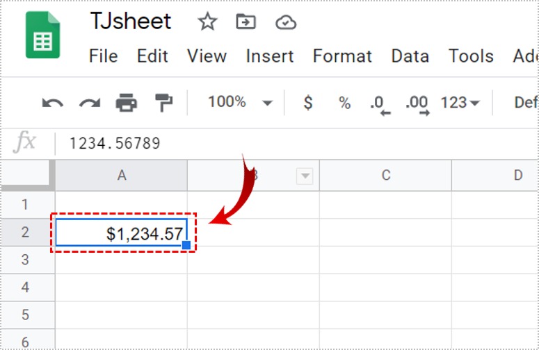
What you should first understand is that although Google Sheets appears to round numbers up or down, it does so only visually. It won’t change the actual value of the inputted number. That said, a cell that’s formatted as currency will always show two decimal places by default, unless it’s custom formatted.
Disable Rounding in Google Sheets using the TRUNC() Function
TRUNC(), or Truncate, is a function built into Google Sheets that allows the display of decimal places without rounding up or down. Any decimal places not displayed retain their value, they’re just not shown. This is the simplest method of showing exact numbers without having to define a custom number format.
Its use is also quite simple. Just type the script into a cell where you want the un-rounded number to be displayed. The Syntax of the code is as follows:
- The code is ‘=TRUNC(Value,[Places])’ where:
- ‘=’ is the command line telling Google Sheets that this is a format script.
- ‘TRUNC’ is the command that determines that whatever is entered is to be truncated.
- ‘Value’ is the amount that you wish to show that will not be rounded
- ‘Places’ is the number of decimals you wish shown.
For example: if you wish to display 123.45678 without rounding up or down, the code will be =TRUNC(123.45678,5).
- In a new Google Sheet, enter ‘=TRUNC(123.45678,3)‘ and hit Enter.

- Of course, you can enter variables in the value section so you won’t have to enter numbers manually. For example, if you wish to truncate the value of the number in cell A1 showing up to five decimals, the formula would be =TRUNC(A1,5). If you wish to display the truncated value of the sum of two cells, you can input the process as =TRUNC(A1+A2,5).

- The value can also be another script. For example, the sum of several cells, A1 to A10 will be written as =SUM(A1:A10). If you want to show it truncated to six decimal places, the formula would be =TRUNC(SUM(A1:A10),6). Just omit the equals sign for the second process so you don’t get an error.
- The value can also be a number located in another sheet. For example, you want to show the truncated value of a number on cell A1 of Sheet 2 up to five decimal places. You can type the formula as =TRUNC(Sheet2!A1,5). The ‘!’ is an indicator that the data you’re trying to get is in another sheet. If the other sheet has been renamed, for example, products instead of sheet2, then you would enter the formula as =TRUNC(products!A1,5) instead.


Be careful of the syntax that you use when typing in the formula. The code may not be case sensitive, but misplacing a comma or a parenthesis will cause the function to return an error. If you’re getting a #NAME error, it means that Google Sheets is having trouble locating a value that you entered. Check your code by clicking on it and looking at the value window just above the sheets. This is the long text box with fx to the right of it. If a cell has a formula, it will always be displayed here.
Formatting Currencies in Google Sheets
As said beforehand, any cell formatted to display currencies will only show up to two decimal places unless formatted otherwise. Doing this is rather simple, but won’t be obvious to those who don’t use Sheets regularly.
To format a cell to display more than two decimals not rounded up or down, do the following:
- Click on the cell you want to format.
- Click on Format menu on the top menu bar.
- Hover over Number to display further options.
- Hover over More Formats at the bottom of the menu.
- Click on Custom number format.
- Enter the number format you wish to use. The list of number formats will display several types, and how the numbers will be displayed if you use each type. If you want to use a currency format just type ‘$’ before the hashtags. For example, if you want to display a currency with a thousand separator with up to three decimals, type in ‘$#,####.###’.
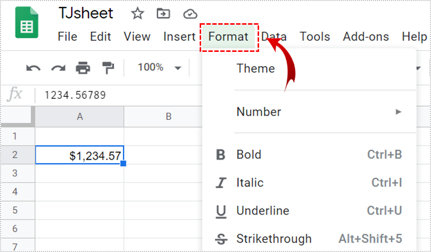


Each hashtag represents a potential number. Increase or decrease the number of hashtags as you see fit.
- If you want to use different currencies when hovering over More Formats, choose More Currencies instead of Custom number format.
- Change the currency you’re currently using, then proceed to change the Custom number format as indicated in the instructions above.

Google Sheets and Preventing Rounding
Getting the exact values of numbers in Google Sheets is quite simple if you know how. TRUNC(), and the Custom number format options, may not be immediately obvious to a casual user, but they’re great tools to have.
Do you have other tips on how to stop Google Sheets rounding certain numbers? Share your thoughts in the comments section below.
Disclaimer: Some pages on this site may include an affiliate link. This does not effect our editorial in any way.