How to Multiply Two Columns in Google Sheets

Learning how to use formulas in Google Sheets can help you calculate data more efficiently. It can also save you a lot of time, especially when you need to multiply two columns. However, these formulas can seem complicated. But once you get a grasp of them, they’ll make your life so much easier.

In this article, we’ll show you how to use a formula to multiply two columns in Google Sheets and other multiplying functions.

Basics of a Multiplication Formula

For a formula in Google Sheets to work, it should have some signs you have to remember. The first one, which is the basis of every formula, is an equality sign (=). For your formula to be valid and to show numbers, write this sign at the beginning.

Next, to multiply numbers, you’ll use an asterisk sign (*) between them. Finally, to get the sum and complete your formula, press ‘Enter.’

Multiplying Two Columns

To multiply two columns in Google Sheets, you’ll first have to insert data. The most efficient way is to use an Array Formula.

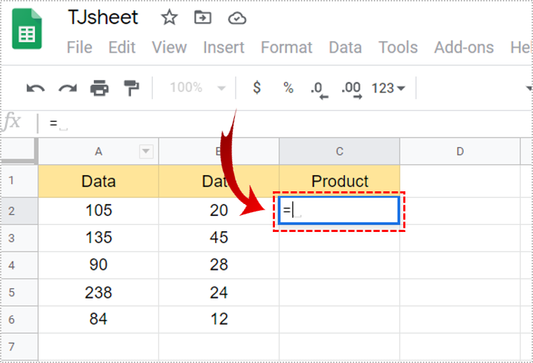
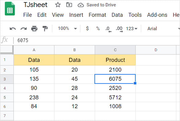
Let’s assume you want to have a multiplied value of data from columns A and B. Select the cell where you want the sum to appear. Follow these steps to successfully apply the formula:

1. First, write an equal sign (=) in the selected cell.
   
   
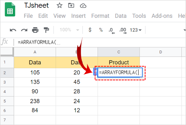
2. Next, type ARRAYFORMULA(.
   
   
3. Alternatively, you could press Ctrl + Shift + Enter, or Cmd + Shift + Enter for Mac users. Google Sheets automatically adds an array formula. Replace ‘)’ by ‘(’ at the end of the formula and follow the next step.
   
   
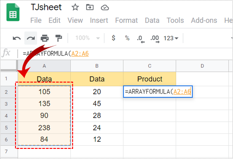
4. Now, drag down the cells in the first column you want to multiply.
   
   
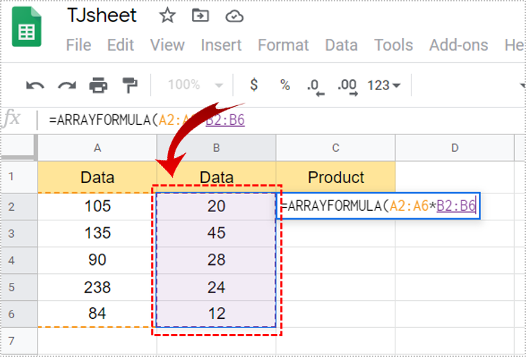
5. Then, type ‘*’ to make sure you’re multiplying.
   
   
6. Drag down cells from the other column.
   
   
7. Finally, tap ‘Enter’ to apply the formula.
   
   
8. The column you selected will show the multiplied values.
   

Once you create an Array Formula, you can’t delete or edit an individual array. However, you can remove an array altogether. Just double-click on the cell where you typed the formula and delete the content. It’ll automatically remove all sums from the column.

Getting a Sum of Multiplied Values

If you need to get a sum of multiplied values for some reason, there’s also a simple way to do it. Just make sure you go through these steps:

1. First, complete the steps above to multiply the cells.
2. Now, select the cell where you want to get the sum of the multiplied value.
3. Type an equality sign (=) there.
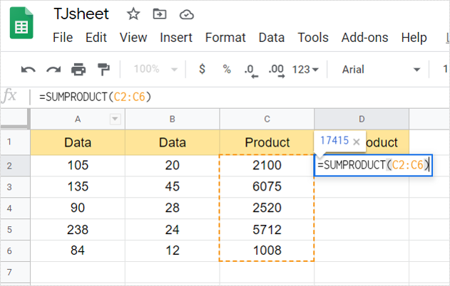
4. Next, write ‘SUMPRODUCT(’.
5. Then, select the cells you want to sum. (These are going to be the cells with your Array Formula).
6. Finally, click ‘Enter’ to get the sum.

Multiplying Across Columns

When you have two separate columns with data, and you need to multiply them, follow these steps:

1. First, select the cell where you want the sum to appear.
2. Type an equality sign (=).
3. Then, click on the cell from the first column.
4. Now type ‘*.’
5. Next, select the cell from the other column.
6. Finally, tap ‘Enter.’
7. The number will appear in the cell you selected.

To have all values appear in the column, click on the small square in the bottom right corner of the multiplied value. You should be able to drag it down the column. This way, all products will show in the cells.

Multiplying with the Same Number

If you have to multiply cells with the same number, there’s a special formula for that, as well. You’ll have to use something called an absolute reference. This is represented by a dollar symbol ($). Take a look at this Google Sheet. There are some data in the A column, which we want to multiply by three.

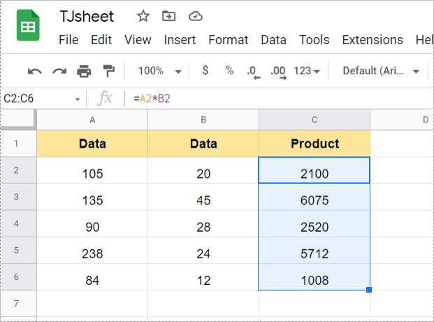
But we don’t want to do it manually for every cell. It’s time-consuming, especially if there are a lot more cells with numbers than we have here. To multiply A2 with B2, you just have to type the following:

1. In the cell you want to have the multiplied value, write an equality sign (=). We’ll type that in C2.
2. Now, either click on A2 or type it next to ‘=.’
3. Then, write ‘*.’
4. After that, click on B2 or type it.
5. Tap ‘Enter.’
6. The number should appear where you want it.

Now, you might try to drag down the value to get the multiplied value for all cells. Unfortunately, this won’t work and you’ll just get zero in all cells.

For the product to show across cells, you’ll have to apply a different formula. That’s why you’ll have to use an absolute reference. Although it sounds complicated, it isn’t. Bear with us.

1. Select the cell where you want the value to appear.
2. Now, write down an equality sign (=).
3. Click on the cell you want to multiply.
4. Type ‘*.’
5. Next, click on the cell you want to use to multiply all cells. For example, B2.
6. Insert ‘$’ in front of the letter and the number representing. It should look like this ‘$B$2.’
7. Tap ‘Enter’ to finish the formula.
8. Click on the small square in the bottom right corner of the formula.
9. Drag it down the column for values to appear in all cells.

When you write ‘$’ in front of the letter and the number representing the cell, you’re telling Google Sheets it’s an absolute reference. So when you drag down the formula, all values represent the multiplication of that number and other numbers from the cells.

Use Google Sheets for Advanced Calculations

Google Sheets can be so useful for advanced calculations. However, it can be tricky if you don’t know which formulas to use. In this article, we’ve outlined how to multiply two columns and perform other multiplying operations.

Do you use Google Sheets for multiplying? Which of the methods in this article do you use the most? Let us know in the comments section below.