Finding data in a spreadsheet can be a nightmare if it’s not organized efficiently. Fortunately, Microsoft Excel spreadsheets give users a way to organize and alphabetize in ascending or descending order. You can also specify the alphabetization in rows or columns.
While alphabetization may not work with some data, it can work wonders to streamline information containing names, addresses, and categories.
The article below will discuss the different ways and methods of alphabetizing your data in Excel.
Alphabetizing a Column in Microsoft Excel
You can utilize the quick sort option in Excel to sort your data in ascending or descending order. This method allows your table to remain comprehensive and complete by moving the data into the appropriate columns. Find the quick sort preference described below:
- Open the Microsoft Excel spreadsheet.
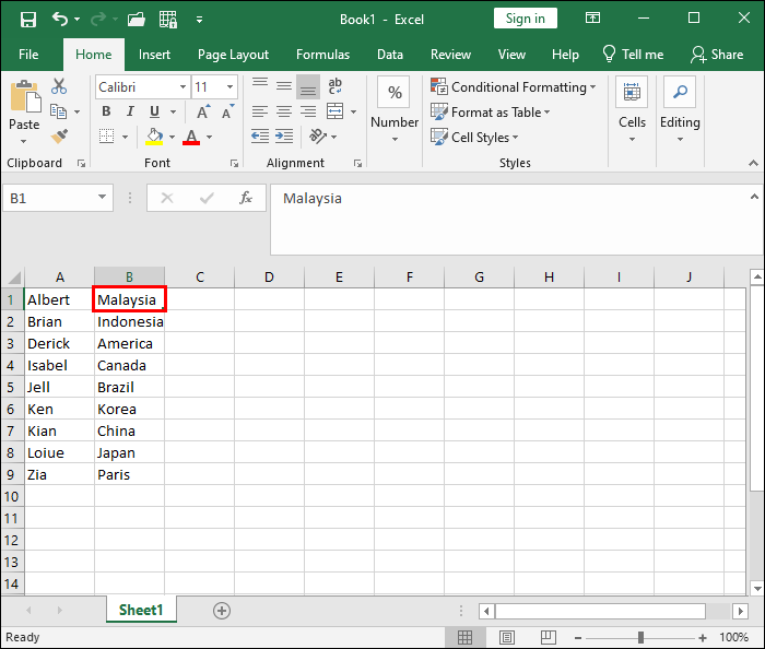
- Choose the column that contains the data you’d like to alphabetize and select the header of that specific column.

- Go to the ribbon at the top of the screen and select the tab for “Data.”
- Select “Sort and Filter.”
- If you’d like to sort your data in ascending order, then select the “ZA” (Z to A) option. If you’d like to sort your data in descending order, then select the “AZ” (A to Z) option.


After the above, all the data in your spreadsheet will be alphabetized according to the option you chose (ascending or descending).
Alphabetizing a Row in Microsoft Excel
The quick sort option allows you to sort your data into columns but doesn’t stop there. You can also sort the data and alphabetize it in a row. This option is pretty similar to the steps for alphabetizing in columns, with the difference of an additional step:
- Launch your spreadsheet in Microsoft Excel.
- Choose the table with the data you want to alphabetize and click on the entire table, excluding the table’s header.
- Select the “Data” tab from the spreadsheet ribbon.
- Go to “Sort and Filter” and select “Sort.”
- Once you’re in the “Sort” window, go to the top of your screen and select “Options.”
- Click “Sort Left to Right” and then confirm the action.
- Select “Order” for another drop-down table, and then click on “A to Z” or “Z to A” in order to complete the alphabetizing of your row.


Alphabetizing Your Data in Excel via the Filter Button
This article has outlined the quick sort option for alphabetizing your data. However, you can use another method through the “Filter” button. The filter approach offers more convenience as it combines all the options and simply awaits your confirmation. It’s much quicker and requires less steps:
- Open the spreadsheet to the set of data you’d like to alphabetize.
- Select the column headers of the data set to filter.
- Go to the top of the screen and select the “Data” tab and the “Filter” option.
- You’ll see a tiny drop-down arrow (at the bottom right corner) on each column header you selected.
- Select these arrows for another drop-down menu.
- Choose whichever option you’d prefer to alphabetize your data.


Using The “SORT” Function to Alphabetize Your Data
There is an additional way to alphabetize your data: by using the “SORT” function. This method might appear slightly daunting initially, but it is fairly straightforward once you get the hang of the steps. However, it’s important to understand what each component means and what it stands for before getting into the steps.
The “SORT” function is composed of:
- Array – This applies to the range that you’d like to sort.
- sort_index1 – This refers to the specific row or column that you’d like to organize.
- sort_order1 – This applies to the desired order in which you’d like to sort your data (e.g., ascending or descending order).
- sort_index2 – This applies to the column you’d like to organize by adding more levels.
- sort_order2 – This applies to the sorting organization for Level 2.
When utilizing the SORT function, it’s important to note that the above components are all optional except for the array. If you don’t specify a particular sort order, you can add as many levels as you’d like, with a maximum of 128. Excel will sort it into ascending order by default.
FAQs
Is there a shortcut to arranging data alphabetically in Microsoft Excel?
Yes. If you’d like to arrange your data alphabetically, use the “Alt + Shift + S” shortcut to access the “Sort Dialog” box. Choose the column you’d like to organize and the order in which you’d like to arrange your data. Once this step is complete, you can confirm by clicking “OK.”
We Love to Excel
Trying to find pertinent data in spreadsheets can be a frustrating and time-consuming endeavor. Fortunately, Microsoft Excel has simplified sorting options for its users. From basic filtering to more advanced methods, you can choose the level of sorting that meets your preferences. And if you’re feeling particularly adventurous or want to be an Excel master, you can try out the “SORT” method. Just be sure to save a copy first, just in case!
What’s your favorite method of sorting and filtering spreadsheets? Do you go with the tried and true ribbon method, or do you use more advanced techniques? Tell us about it in the comments section below.
Disclaimer: Some pages on this site may include an affiliate link. This does not effect our editorial in any way.