How To Round Google Sheets Cells to the Nearest 10

Gregory Read more May 18, 2021

The MROUND function in Google Spreadsheets provides a simplistic way to round a number either upwards or downwards to the nearest 0.5, 5, 10, or any other specified multiple you choose. An example of this is using the function to round up or down an item’s total cost the nearest cent. This could be five cents (0.05), ten cents (0.1), or even twenty five cents (0.25) if so inclined. This helps avoid off numbers resulting in pennies on the dollar by rounding three cents (0.03) up to five or thirty three cents (0.33) down to a quarter when providing change.

How To Round Google Sheets Cells to the Nearest 10

Unlike using formatting function keys that allow you to alter the decimal places shown without actually changing a cell’s value, the MROUND function will actually alter the value of the data. By using this function to round your data to a specified amount, the calculated results will be affected. If you’d prefer to not specify a number for rounding, you can instead utilize the ROUNDUP or ROUNDDOWN functions.

Syntax and Arguments of the MROUND Function

A function’s syntax is its layout. This will include the name of the function, the brackets (which are used to index into an array) and the arguments.

The MROUND’s syntax function is:

= MROUND (value, factor)

The arguments available for the function, both of which are required are:

Value: This will be the number that is rounded either up or down to the nearest integer. The argument can use this as the actual data for rounding or it can be used as a cell reference to the actual data already located on the Google worksheet. The value is shown as the number located in the DATA column in the worksheet provided below and is then referenced within each argument to the cell containing the data. In my example, the value/data is 3.27 (referenced as A2), 22.50 (A8), and 22.49 (A9).

Factor: This provides the number by which the value (data) is rounded, either up or down, to the nearest multiple. This is represented by varying degree within my example (0.05, 0.10, -0.05, 10 to name a few).

Examples of the MROUND Function

In the provided image, the first six examples use 3.27 as its value, seen in column A. In all six function cells that value is rounded either up or down by the MROUND function using different integers for the factor argument. The end results are shown in column C with the description of the formula displayed in column D.

The rounding of the last digit or integer is entirely dependent on the value argument. If the value’s rounding digit and all numbers to the right are less than or half of the factor argument, the function will round down. If those same numbers are greater or equal to the factor argument, then the digit is rounded up.

Rows 8 and 9 are a prime example for demonstrating how the function handles rounding both up and down. Both rows have single digit integer, which in this case is 5. This means the second 2 for both row 8 and 9 becomes the rounding digit. Since 2.50 is equal to half the value of the factor argument, the function is rounded up to 25, the nearest multiple of 5. Where as in row 9, 2.49 is less than half the value of the factor argument, and is rounded down.

How To Enter the MROUND Function

Google sheets uses an auto-suggest box when entering a function into a cell. This can be a bit annoying when you don’t mean to enter a function but there really isn’t much of a workaround. To enter the MROUND function I’ve created in my example:

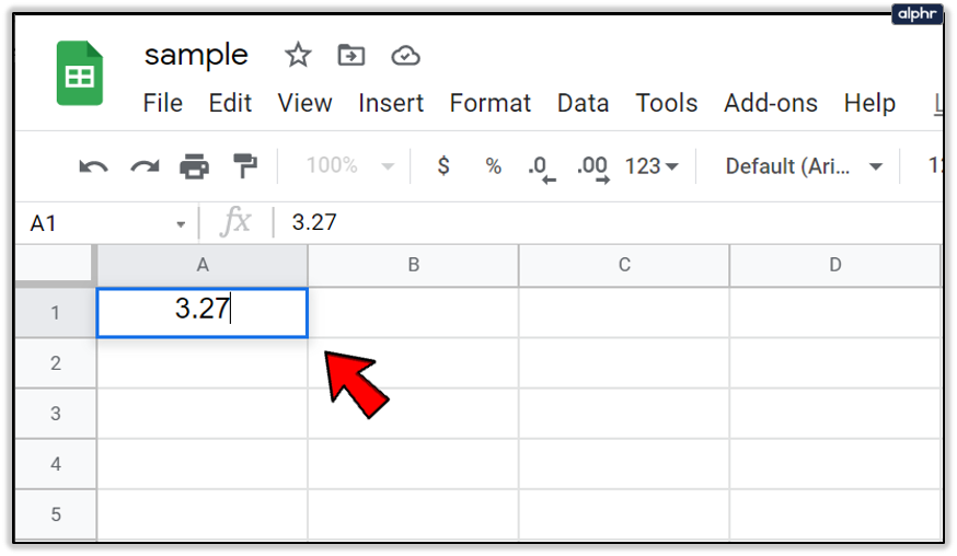
Type 3.27 into cell A1 of your Google Sheet.
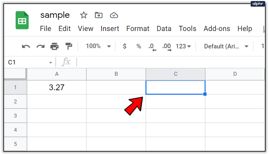
Click to highlight cell C1 as this will be your active cell where the results are generated.
Hit the ‘=‘ key followed by typing in MROUND. You’ll see the auto-suggest box pop up with the name of the function. When this occurs, you can click on the function in the box to automatically place a bracket or you can type them in yourself.
Now click on A1 to enter this cell reference as your value argument.
Follow this up by typing in a comma to separate the arguments, and then type 0.05.
You can end the argument with a follow up bracket or simply press Enter on the keyboard for it to auto-complete.

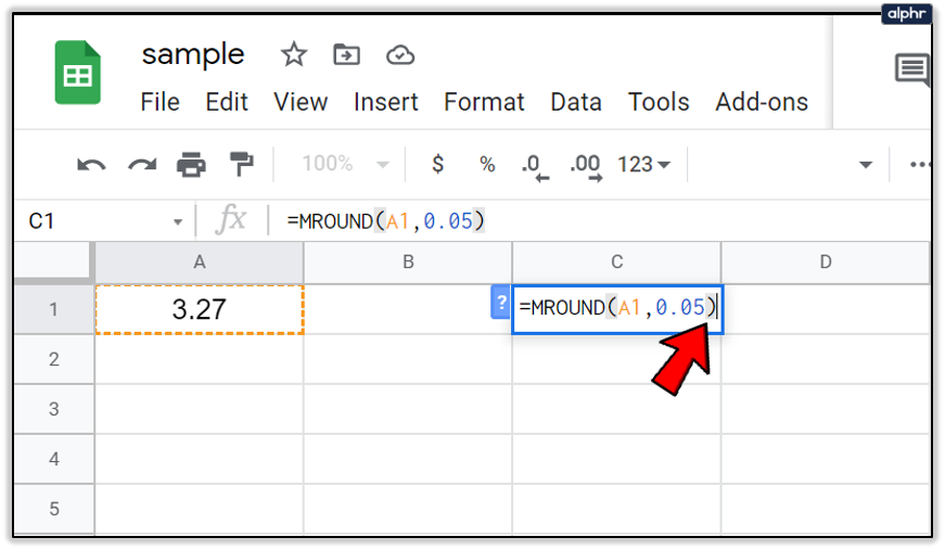
The value should now show as 3.25 since the value was rounded down to the nearest 0.05. The function itself will disappear leaving only the current value, however, you can also view the complete function as written by highlighting cell C1 and glancing at the formula bar.