Over the past few years, Google Sheets has established itself as one of the most versatile data analysis tools on the market. From managing personal finances to creating detailed charts and graphs for business analysis, Google spreadsheets can do it all.
One feature that most users often overlook is the incorporation of the current date into spreadsheets. Adding the current date to your Google Sheets can help you track changes, overdue tasks, and even perform calculations that are linked to time.
In this article, we take an in-depth look at the ways you can use the current date in Google Sheets to streamline your workflow, enhance your spreadsheets, and stay on top of time-sensitive tasks.
The Today Function in Google Sheets
The Today function is programmed to return today’s date on your spreadsheet. The best thing about it is that it updates automatically whenever the sheet recalculates, so you don’t have to change the date manually every time you reopen your work.

Unlike most Google Sheets functions, the Today function doesn’t require complex arguments. All you need is to enter “=TODAY()” in the cell of interest. Let’s look at a few applications of this function to help understand how to use it on your spreadsheets.
Tracking Deadlines
Suppose you have listed different projects on your spreadsheet where each project has its own deadline. For example, assume the deadline for project A is in cell A1. To calculate the number of days remaining until the deadline, you’d need to enter the following formula in the relevant cell:
“=A1 – TODAY()”

This formula will give you the exact number of days between the current day and the deadline. And as with all Google Sheets formulas, you don’t have to enter this information in every cell if the deadlines are in one column. Simply rest your cursor in the lower right corner of the first cell and then drag the fill handle down.
Highlighting Overdue Tasks
The Today function works quite well in conjunction with other formulas and conditional formatting instructions.
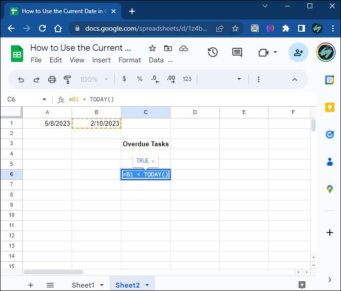
For example, assume you have populated column B with the due date for each project. Using the Today function in conjunction with conditional formatting, you can create a new “Overdue” column that highlights all the projects whose due date happens to be earlier than the current date.
Assuming the first due date is in cell B1, here’s the formula you would need to determine whether the corresponding project is overdue:
“=B1 < TODAY()”
Calculating Age
Assume you have a list of individuals and their dates of birth, and you want to create a column that indicates their ages as of today. For illustration purposes, let’s say the date of birth of the first name on the list is in cell B2. With the following formula, you can easily generate the required data:

“=DATEDIF(A2, TODAY(), “Y”)”
This formula will return the difference between the current date and the date of birth in years.
For example, assume the date of birth in cell B2 is 15/09/1990, and the current date is 29/04/2023. Applying the formula above returns the age as 32. As with all other instances where the Today function is used, the age will update automatically as the current date changes. This means the age column on your document will always be accurate.
Tracking the Last Day of the Month
Now, consider a slightly different scenario where you’re interested in the last day of the month for the current date. Combining the Today function with the EOMONTH function enables you to calculate the end date of the current month almost instantly. This combination also comes with an optional offset to specify the number of months to move forward or backward.

Crucially, the function combines two arguments:
“=EOMONTH(TODAY(), month)”
If you’re wondering how to interpret the function, here’s a brief breakdown:
- “start_date”: This part returns the current date.
- “months”: This is the number of months before or after the current date for which you want the last day. A positive value will move forward in time, with a negative value moving backward.
Let’s quickly look at some applications of the EOMONTH function in conjunction with the current date function:
Finding the Last Day of the Next Month
To find the last day of the next month from the current date, you need to use a positive value for the month argument:

“=EOMONTH(TODAY(), 1)”
Assuming today’s date is May 08, 2023, this formula will return June 30, 2023, which is the last day of the next month.
Finding the Last Day of the Current Quarter
If you want to find the last day of the current quarter, you can use a combination of the EOMONTH and TODAY functions with the CEILING function:

“=EOMONTH(TODAY(), CEILING(MONTH(TODAY()) / 3) * 3 – MONTH(TODAY()))”
If today’s date is May 08, 2023, this formula will return June 30, 2023, which is the last day of the current quarter (May – June).
Finding the Last Day of the Fiscal Year
Suppose your fiscal year ends on March 31, and you want to find the last day of the current fiscal year. You can use the EOMONTH(TODAY(), month) function as follows:

“=IF(MONTH(TODAY()) > 3, EOMONTH(date(YEAR(TODAY()), 3, 31), 12), EOMONTH(date(YEAR(TODAY())-1, 3, 31), 12))”
Again, using May 08, 2023 as the current date, the formula above will return March 31, 2024 as the last day of the current fiscal year.
The Now Function in Google Sheets
Consider a situation where you need to track both the current date and time, for example, when tracking the time to expiration of a highly perishable commodity such as bread. In this case, you’ll need a formula that returns both the current date and time. The Now function gives you just that.
To use it, you just need to enter the following formula in the desired cell:

“=NOW()”
The Options Are Endless
Using the current date in your spreadsheets comes with endless options. You can schedule deadlines, calculate age, and even highlight overdue tasks.
Perhaps the most important thing to remember is that the TODAY and NOW functions are volatile functions, meaning that they recalculate every time the sheet recalculates. In other words, the dates and times indicated will keep on changing as the spreadsheet gets updated. If you want a static date, you can enter it manually or use the shortcut “Ctrl + ;” to insert the current date, and “Ctrl + Shift + ;” to insert the current time.
Have you tried applying any of these handy formulas in your spreadsheets? Feel free to share your experience with other Google Sheets users in the comments.
Disclaimer: Some pages on this site may include an affiliate link. This does not effect our editorial in any way.