How to Calculate Time in Google Sheets

Whether you’re looking to throw together a quick financial spreadsheet or you want to work together with a co-worker on an Excel-like document, Google Sheets is a great web-based, free alternative to Excel.

One of the most valuable aspects of spreadsheet programs is their flexibility. A spreadsheet can serve as a database, calculation engine, platform for statistical modeling, text editor, media library, to-do list, and more. The possibilities are nearly endless. One everyday use for spreadsheets, including Google Sheets, is to track hourly employee time schedules or billable hours.

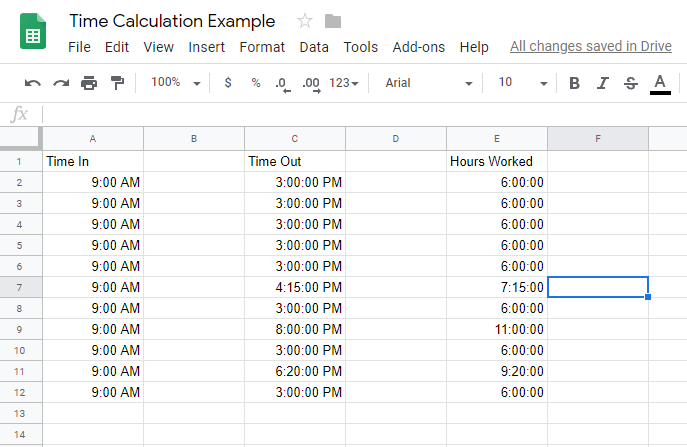
If you are using Google Sheets to track time in this way, you will frequently find yourself needing to calculate the difference between two timestamps (the amount of time passed between two different time events). For example, if someone clocked in at 9:15 AM and then clocked out at 4:30 PM, they were on the clock for 7 hours and 15 minutes. If you need to use Sheets for something like this, you’ll quickly notice that it wasn’t designed to handle these kinds of tasks.

Still, while Google Sheets handles timing log functions, it is easy to persuade it to do with some preparation. This article shows you how to calculate the difference between two timestamps using Google Sheets automatically.

How to Add Times and Calculate Worked Time in Google Sheets

Measuring the difference between two cells containing time data requires that Google Sheets understands that the cells’ data is time data. Otherwise, it calculates the difference between 9:00 AM and 10:00 AM as 100 rather than 60 minutes or one hour. To correctly count time differences, the time columns require formatting as Time and the duration column as Duration.

Furthermore, The calculation is intentionally backward (time out – time in) because it has to account for AM/PM transitions, so you don’t get negative numbers. Therefore, 2:00 PM – 9:00 AM = 5.00 Hours whereas 9:00 AM – 2:00 PM = -5.00 Hours. Test it out if you like.

To make a formatted timesheet showing the time the person started work, the time they left, and the calculated duration worked can be done as follows:

1. Open the specific Google sheet.
   
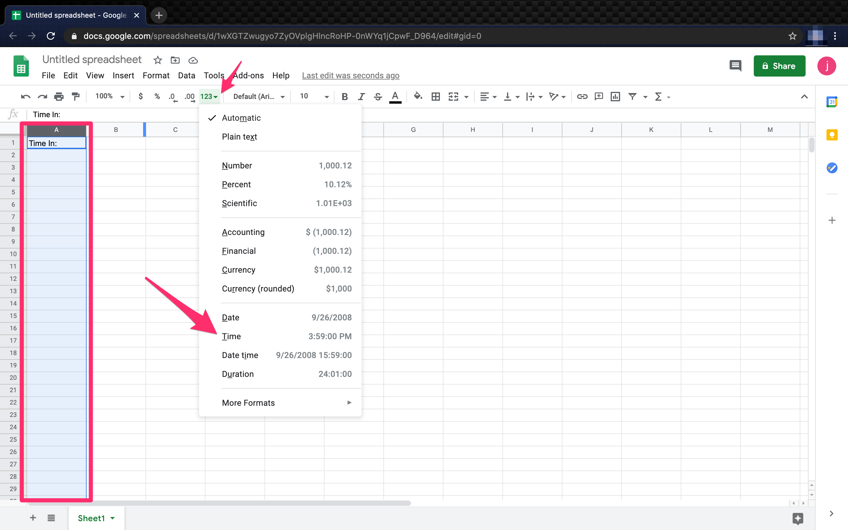
2. Select your Time In: column and click the 123 format drop-down in the menu, then select Time as the format.
   
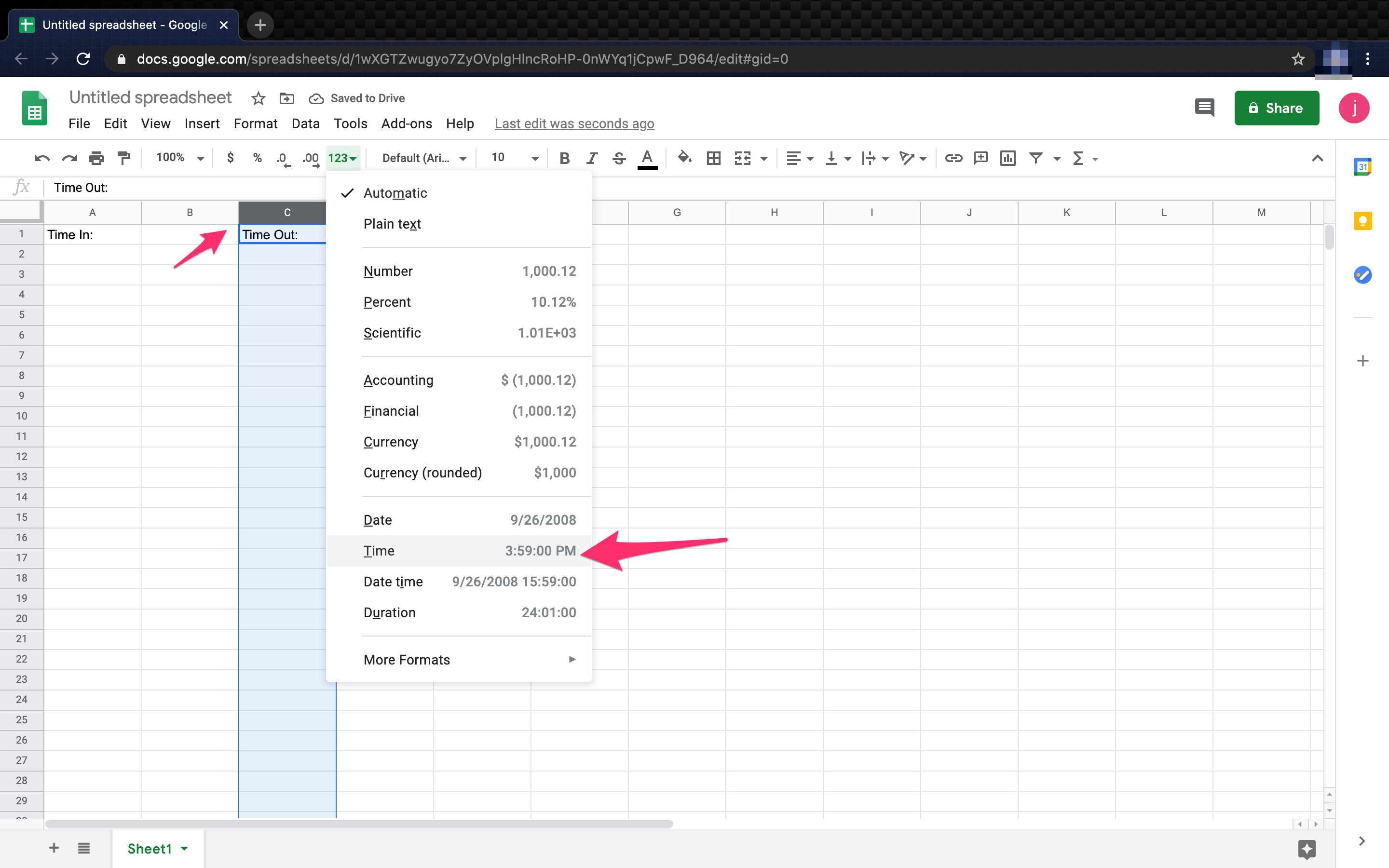
3. Select the Time Out: column, then click on the 123 drop-down menu item, and then select Time.
   
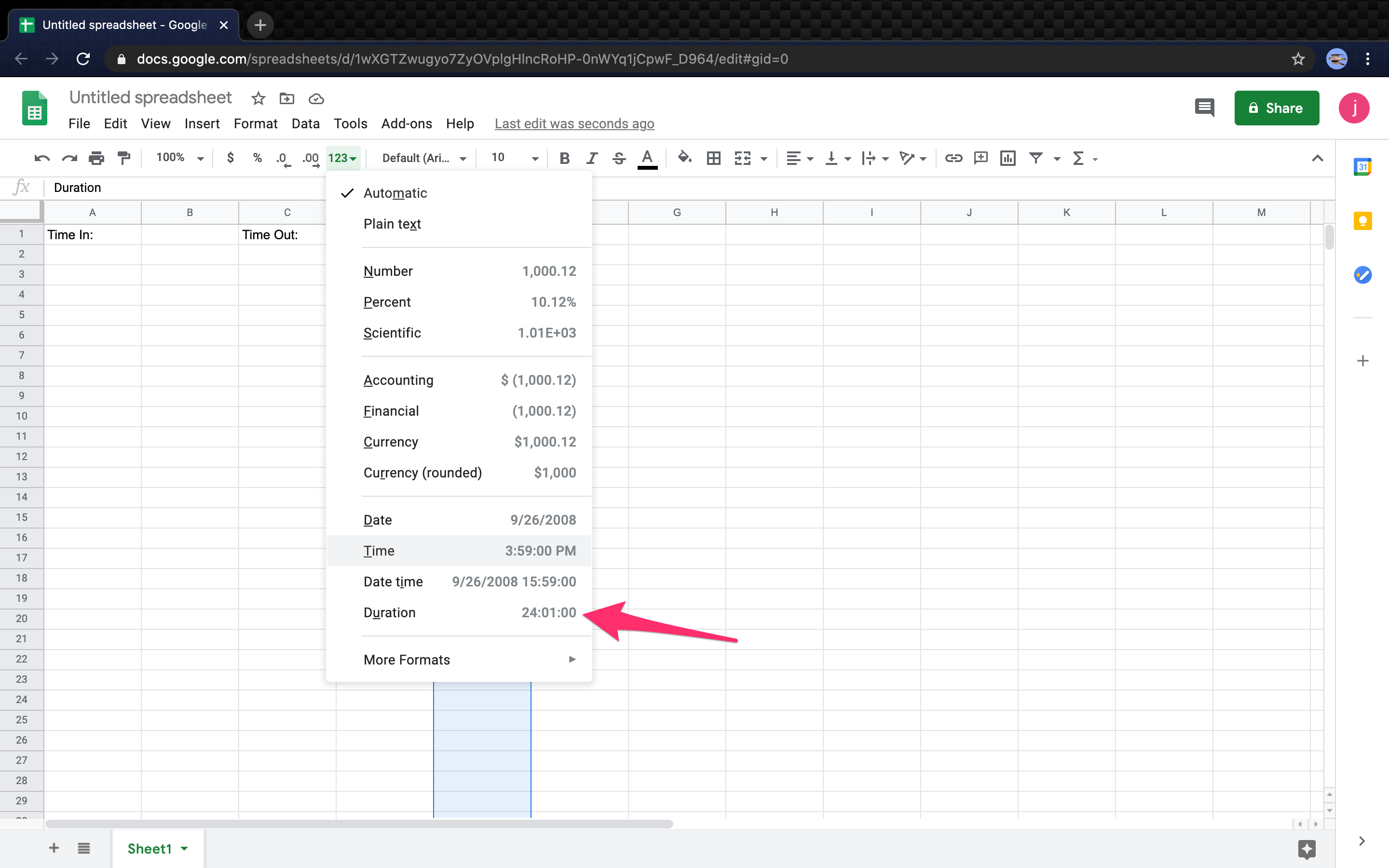
4. Select the Hours Worked: column. Click on the 123 drop-down menu item and choose Duration as the format.
   
5. To activate the formula in the Hours Worked column, type “=(C2-A2)” where C2 represents the Time Out cell, and A2 represents the Time In cell.

That’s all there is to it. Following the steps listed above and using the provided formula is relatively easy to calculate time in Google Sheets. What if you want to add breaks into the calculations? Keep reading to find out.

How to Add Time Gaps or Work Breaks When Calculating Time in Google Sheets

Unless paid lunches or short-term leave are a benefit in the business, you may need to calculate breaks in the worked hours. Even if break times are unpaid time, it works out best to include separate entries versus using “Time In” and “Time Out” for breaks. Here’s how to do it.

Note: Just like basic time in and time out calculations, you need to calculate time in reverse as follows: “Time out” – “Time In,” except you’ll have breaktiume entries in between the formula.

1. Select your Break Out: column and click the 123 format drop-down in the menu, then select Time as the format.
2. Select your Break In: column, click on the 123 format drop-down entry in the menu, and then choose Time as the format.
3. Calculate the hours for the Hours Worked Column. Type “=(C2-A2)+(G2-E2),” which translates to [Break Out (C2) – Time In (A2)] + [Time Out (E2) – Break In (G2)].
4. Use the calculation for every row so that your Hours Worked Column looks like this.
   

How to Add Dates to Your Timesheets in Google Sheets

If you prefer to add dates to the worktime entries, the process is the same as it is for adding time, except you choose Date time as the format instead of Time. Your cells display “MM/DD/YYYY HH/MM/SS” when you choose Date time as the format.

How to Convert Minutes to Decimals in Google Sheets

When dealing with increments of time, it might be helpful to convert them into decimals instead of minutes, i.e., “1 hour and 30 minutes = 1.5 hours.” Converting minutes to decimals is easy; there are several ways to accomplish this.

1. Select the Worked Time column, click on the 123 menu entry at the top, then change the format from Duration to Number. Ignore all the weird characters that appear in the cells.
2. In the first Worked Time cell, copy/type “=(C2-A2)*24+(G2-E2)*24” without quotes. Be sure to change the formula to the correct cell IDs, such as C2-A2.
3. Copy the formula you created in the first Worked Time cell and paste it into all other Worked Time cells in the column. Google autoformats the cells with the correct cell IDs.

In closing, Google Sheets wasn’t explicitly designed to produce timesheets, but it can easily get configured to do just that. This simple setup means you can track hours worked quickly and easily. When timespans cross over the 24-hour mark, things become a little more complicated, but Sheets can still pull it off by changing from Time to Date format.

You can also read our article on calculating how many days have passed between two dates in Sheets.

Google Sheets Time Calculation FAQs

How to find the shortest or highest amount of time worked in Google Sheets?

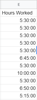
If you quickly need to locate the least amount of time worked, this formula should help. The MIN() function is a built-in function that allows you to find the minimum value in a list of numbers.

1. Create a new cell (I2 in this example) and set the format to “Duration.” Copy/type the function “=MIN(E2:E12)” without quotes and paste it into the cell. Be sure to change the cell IDs, such as “E2.”

Now, the Min. Hours Worked column should show the lowest amount of hours worked, such as 5:15:00.

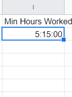
You can easily apply the MIN() or MAX() function to a column or group of cells. Give it a try for yourself.

How to calculate the total hours worked in Google Sheets?

If you’re not familiar with programming or Excel, then some of the built-in functions for Google Sheets may seem strange. Luckily, it doesn’t take much to calculate the total hours worked. In this example, we’ll calculate the total hours worked by all the employees in a day.

1. Create a new cell and assign it Duration.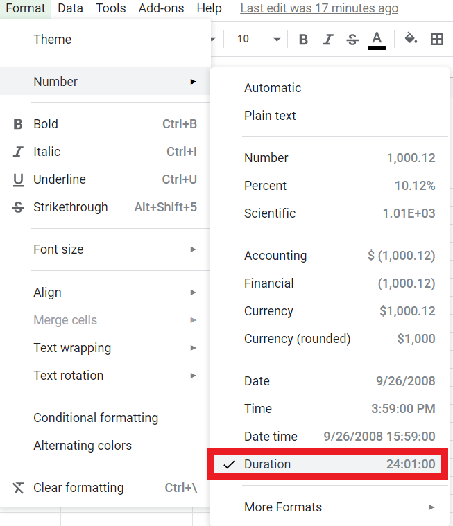

2. In the Formula (fx) Bar: type “=SUM(E2:E12)” without quotes, which provides the total hours worked from cells E2 through E12. This formula is standard syntax for Excel and various programming languages.

The total should appear in the format” 67:20:00″ and look like this: