How To Calculate p-Value in Excel

The theory behind “p-values” and the null hypothesis might seem complicated initially, but understanding the concepts helps you navigate the world of statistics. Unfortunately, these terms often get misused in popular science, so it would be essential for everyone to understand the basics.

Calculating the “p-value” of a model and proving/disproving the null hypothesis is surprisingly simple with MS Excel. There are two ways to do it. Let’s dig in.

Null Hypothesis and p-Value

The null hypothesis is a statement, also referred to as a default position, claiming that the relationship between the observed phenomena is non-existent. The null hypothesis can also apply to associations between two experimental groups. During the research, you test this hypothesis and try to disprove it.

For example, say you want to observe whether a particular fad diet has significant results. The null hypothesis, in this case, is that there is no significant difference in the test subjects’ weight before and after dieting. The alternative hypothesis is that the diet did make a difference. The alternative is what researchers would try to prove.

The “p-value” represents the chance that the statistical summary would be equal to or greater than the observed value when the null hypothesis is valid for a particular statistical model. Though the “p-value” often gets expressed as a decimal number, it is generally better to describe it as a percentage. For example, the “p-value” of 0.1 should get represented as 10%.

A low “p-value” means that the evidence against the null hypothesis is strong. This further means that your data is significant. On the other hand, a high “p-value” means there’s no strong evidence against the hypothesis. To prove that the fad diet works, researchers need to find a low “p-value.”

A statistically significant result is the one that is highly unlikely to happen if the null hypothesis is true. The significance level gets denoted with the Greek letter “alpha,” and it has to be bigger than the “p-value” for the result to be statistically significant.

Many researchers use the “p-value” to get a better and deeper insight into the experiment’s data. Some prominent scientific fields that use “p-value” include sociology, criminal justice, psychology, finance, and economics.

Finding the p-Value in Excel 2010

You can find the “p-value” of a data set in MS Excel via the “T-Test” function or using the “Data Analysis” tool. First, we’ll look into the “T-Test” function. You’ll see five college students that went on a 30-day diet and comparable data on their weight before and after the diet.

NOTE: This article covers p-value functionality for MS Excel 2010 and 2016, but the steps should generally apply to all versions. However, the graphical user interface (GUI) layout of the menus and whatnot will differ.

T-Test Function

Follow these steps to calculate the “p-value” with the T-Test function.

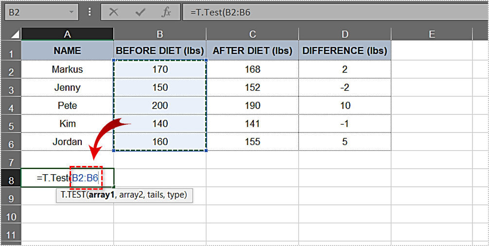
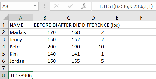
1. Create and populate the table. Our table looks like this:
   
2. Click on any cell outside your table.
   
3. Type”=T.Test(“(include the starting parenthesis) into the cell.
   
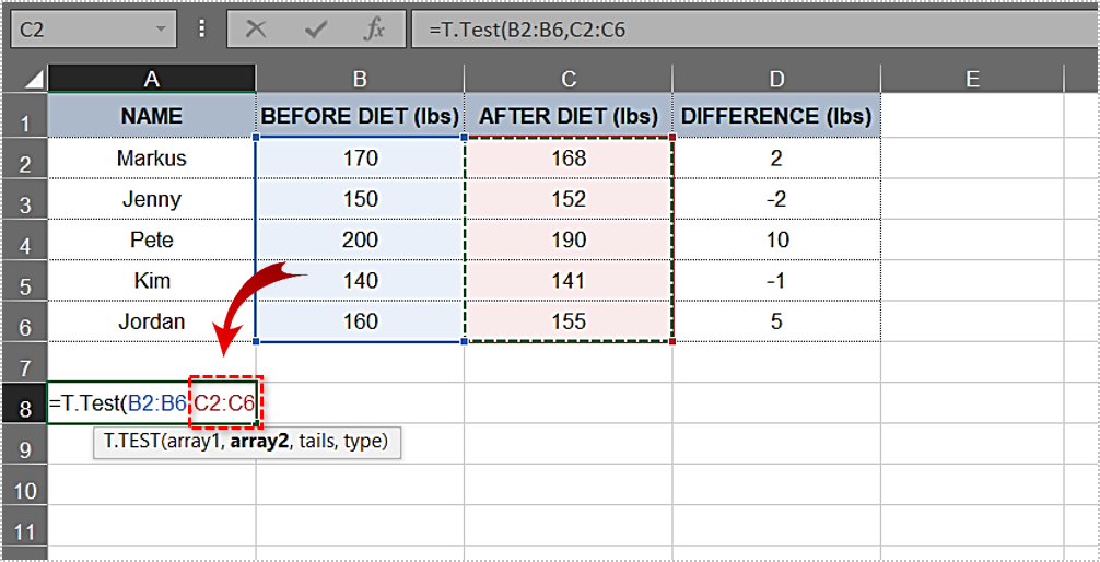
4. After the starting parenthesis, type in the first argument. In this example, it is the “Before Diet” column. The range should be”B2:B6.” Thus far, the function looks like this: T.Test(B2:B6.
   
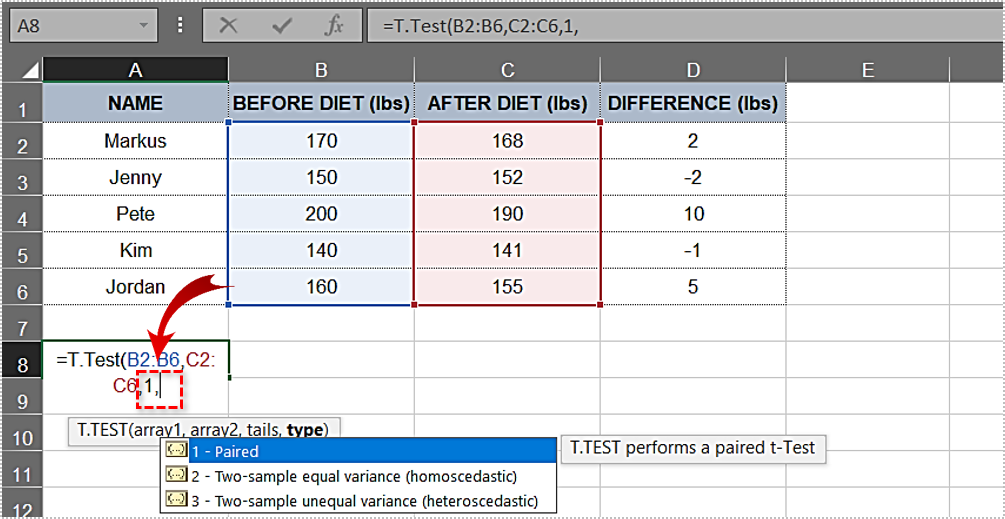
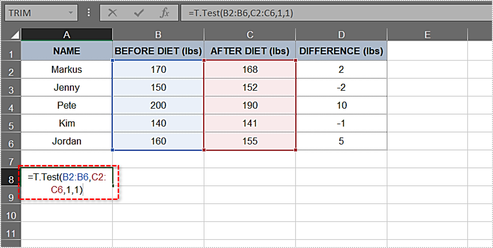
5. Next, enter the second argument. The “After Diet” column, along with its results, is the second argument, and the range you need is the following: “C2:C6.” Let’s add it to the formula: T.Test(B2:B6,C2:C6.

6. Type in a comma after the second argument. The one-tailed distribution and two-tailed distribution options automatically appear in a drop-down menu. Go ahead and choose "one-tailed distribution" by double-clicking on it.

7. Type in another comma. For ease of use, the complete code is listed further down.

8. Double-click on the "Paired" option in the following drop-down menu.
   
9. Now that you have all the needed elements, you need to insert an ending parenthesis. The formula for this example looks like this: =T.Test(B2:B6,C2:C6,1,1)
   
10. Press “Enter.” The cell now displays the “p-value” immediately. In our case, the value is “0.133905569” or “13.3905569%.”
    

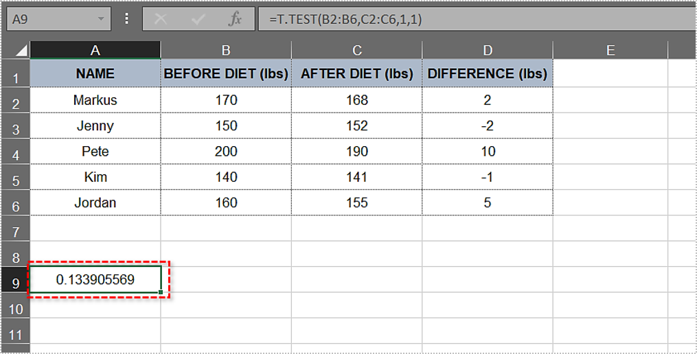
Being higher than 5%, this “p-value” doesn’t provide strong evidence against the null hypothesis. In our example, the research didn’t prove that dieting helped the test subjects lose significant weight. The results don’t necessarily mean the null hypothesis is correct, only that it hasn’t been disproven yet.

Data Analysis Route

The “Data Analysis” tool lets you do many cool things, including “p-value” calculations. We’ll use the same table as the previous method to simplify the process.

Here’s how to use the “Data Analysis” tool.

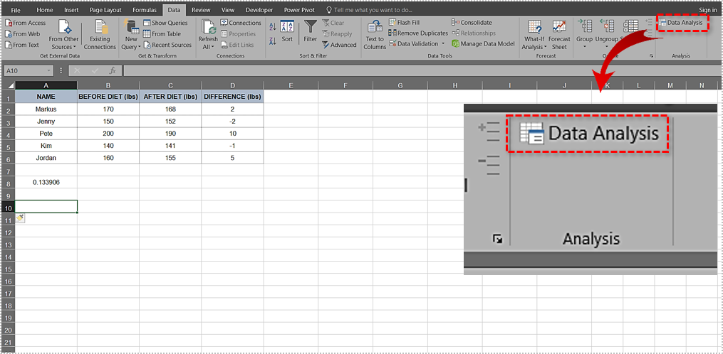
1. Since we already have the “weight” differences in the “D” column, we’ll skip the difference calculation. For the future tables, use this formula: =”Cell 1”-“Cell 2”.
2. Next, click on the “Data” tab in the Main menu.
   
3. Select the “Data Analysis” tool.
   
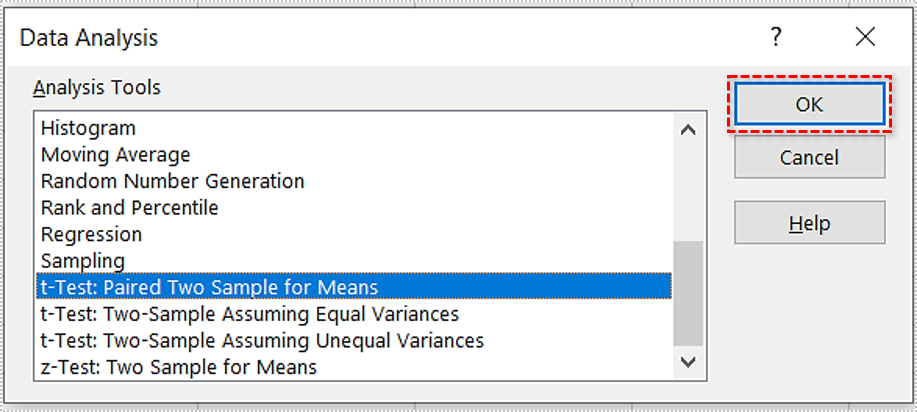
4. Scroll down the list and select “t-Test: Paired Two Sample for Means.”
   
5. Click “OK.”
   
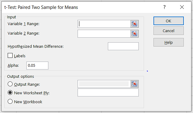
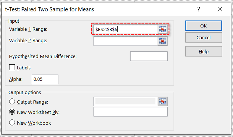
6. A pop-up window appears. It looks like this:
   
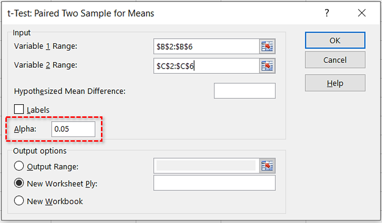
7. Enter the first range/argument. In our example, it is “$B$2:$B$6“as in “B2:B6.”
   
8. Enter the second range/argument. In this case, it is “$C$2:$C$6“as in “C2:C6.”
   
9. Leave the default value in the “Alpha” text box (0.05).
   
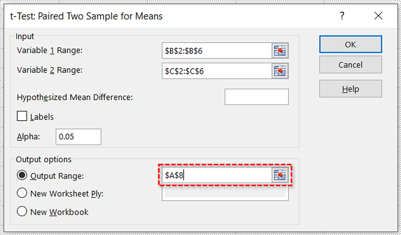
10. Click on the “Output Range” radio button and pick where you want the result. If it’s the “A8″ cell, type the following:”$A$8.”
    
11. Click “OK.”
    
12. Excel will calculate the “p-value” and several other parameters. The final table might look like this:
    

As you can see, the one-tail “p-value” is the same as in the first case (0.133905569). Since it is above 0.05, the null hypothesis applies to this table, and the evidence against it is weak.

Finding the p-Value in Excel 2016

Like the steps above, let’s cover calculating the “p-Value” in Excel 2016.

1. We’ll use the same example above, so create the table if you want to follow along.
2. Now, in Cell “A8,” type the following: =T.Test(B2:B6, C2:C6.
3. Next, in cell A8, enter a “comma” after “C6” and then select “One-tailed distribution.”
4. Then, enter another “comma” and select “Paired.”
5. The equation should now be the following: =T.Test(B2:B6, C2:C6,1,1).
6. Finally, press “Enter” to show the result.

The results may vary by a few decimal places depending upon your settings and available screen space.

Things to Know About the p-Value

Here are some valuable tips regarding “p-value” calculations in Excel.

1. If the “p-value” is equal to 0.05 (5%), the data in your table is “significant.” If it is less than 0.05 (5%), the data is “highly significant.”
2. In case the “p-value” is more than 0.1 (10%), the data in your table is “insignificant.” If it’s in the 0.05-0.10 range, you have “marginally significant” data.
3. You can change the “alpha” value, though the most common options are 0.05 (5%) and 0.10 (10%).
4. Depending on your hypothesis, “two-tailed testing” can be the better choice. In the example above, “one-tailed testing” means we explore whether the test subjects lost weight after dieting, which is what we needed to find out precisely. But a “two-tailed” test would also examine whether they gained significant weight.
5. The “p-value” can’t identify variables. In other words, if it finds a correlation, it can’t recognize the causes behind it.

p-Value Demystified

Every statistician must know the ins and outs of null hypothesis testing and what “p-value” means. This knowledge also comes in handy to researchers in many other fields.