How To Automatically Adjust Row Height in Excel

If you deal with long numbers, names, formulas or something that won’t generally fit into a standard cell, you can manually stretch the dimensions of that cell to fit. But wouldn’t it be cool if you could automatically adjust row height in Excel? You can and this tutorial will show you how.

There are lots of things you can do with cells and I’ll cover a few of those too.

Usually if your data doesn’t fit into the cell, Excel will show the first few characters and then run the content across other cells so you can read it all. If there is data in those other cells, you don’t get to see this information so this is where automatic adjustment comes in useful.

Autofit in Excel

You likely already know to drag and stretch cells, columns and rows to manually resize them. You may even know how to select multiple cells and stretch those or even the entire spreadsheet to resize all cells to fit the largest cell data. But did you know you can automatically adjust row height and column width?

It’s actually very straightforward.

Adjust row height in Excel

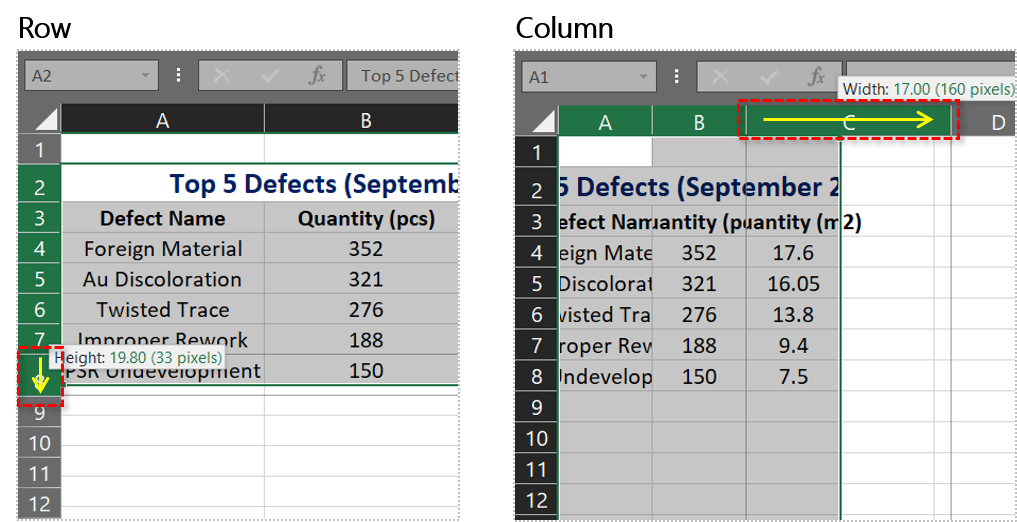
To adjust row height in Excel, add your cell data as you normally would and you will likely see some of it cut off from view. To automatically adjust the row height, just double click the border of the cell in question.

For row height, double click the bottom border of the row number on the left of the spreadsheet. The cursor will change to a line with an up and down arrow either side. The spreadsheet will now automatically adjust the selected row to hold the data while showing it all.

Adjust column width in Excel

To adjust column width in Excel, you do the same thing but on each side of the cell. To automatically have Excel adjust the width of a column, double click on the right of the column header. As with row height, the cursor should change to a line with arrows either side. Double click when the cursor is like this and the column will automatically adjust.

Adjust multiple rows or columns in Excel

You can also adjust multiple rows or columns at once in Excel. If you have a large spreadsheet with a lot going on, manually adjusting each one to fit your data could take forever. Fortunately, there’s a shortcut you can use to adjust multiple at once.

1. Select a row or column header in your spreadsheet.
   
2. Hold Shift and select all the rows or columns you want to adjust.
   
3. Drag one border to the size you want it.
   

For example, you want to widen columns to fit in your data. You select multiple columns as above, say A, B and C. Drag the column header of C to the right to make them wider and all three columns will move to reflect the new size.

The same for row height. Select rows 2 to 8 and drag the border down. It will be reflected in all seven rows at once.

Adjust the entire spreadsheet to fit cell data

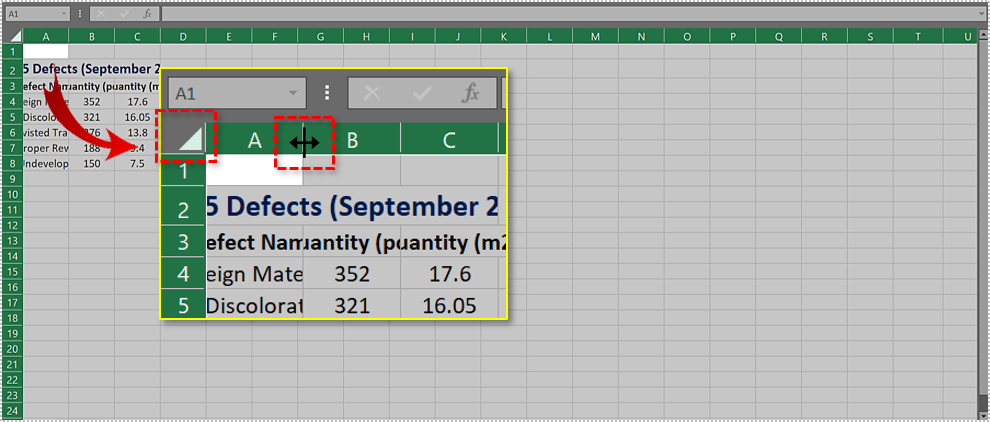
If adjusting individual or multiple rows or columns would take too long, you can have Excel automatically adjust the entire spreadsheet for you. Select the corner arrow of your spreadsheet to select all of it. Double click one column border to automatically adjust the entire spreadsheet to fit.

Specify row height and cell width in Excel

You can also manually configure specific row heights and cell widths in Excel. This is useful for presentations or when an ordered spreadsheet is more important than a flexible one.

1. In Home tab, select Format in Cells group.
2. Select Row Height and/or Column Width.
3. Set a size in the popup box. It is in centimeters.
4. Select OK to save.

You will likely need to adjust this to fit but if you’re presenting or using a spreadsheet as a display, this may offer a more ordered look than your typical spreadsheet.

Using word wrap in Excel

If you have text-based cells that are throwing off your appearance, you can use word wrap to tidy it up a little. Like most word wrap functions, this will cause the text to remain within the border and flow line after line. This can be useful for longer cells such as product names, addresses and longform data.

1. Open your spreadsheet and select the Home tab.
2. Select Format from the ribbon and Format Cells from the menu.
3. Select the Alignment tab from the popup window.
4. Check the box next to Wrap Text.

Now instead of text running over other columns, it will stay within its own column border and flow downwards instead of across your spreadsheet.